http://www.scirp.org/journal/ojop ISSN Online: 2325-7091
ISSN Print: 2325-7105
A New Approach for Solving Linear Fractional
Programming Problems with Duality Concept
Farhana Ahmed Simi
1, Md. Shahjalal Talukder
21Department of Mathematics, Dhaka University, Dhaka, Bangladesh
2Department of Natural Sciences, Daffodil International University, Dhaka, Bangladesh
Abstract
Most of the current methods for solving linear fractional programming (LFP) problems depend on the simplex type method. In this paper, we present a new approach for solving linear fractional programming problem in which the ob-jective function is a linear fractional function, while constraint functions are in the form of linear inequalities. This approach does not depend on the simplex type method. Here first we transform this LFP problem into linear programming (LP) problem and hence solve this problem algebraically using the concept of duality. Two simple examples to illustrate our algorithm are given. And also we compare this approach with other available methods for solving LFP problems.
Keywords
Linear Fractional Programming, Linear Programming, Duality
1. Introduction
The linear fractional programming (LFP) problem has attracted the interest of many researches due to its application in many important fields such as produc-tion planning, financial and corporate planning, health care and hospital planning. Several methods were suggested for solving LFP problem such as the variable transformation method introduced by Charnes and Cooper [1] and the updated objective function method introduced by Bitran and Novaes [2]. The first me-thod transforms the LFP problem into an equivalent linear programming prob-lem and uses the variable transformation y=tx t, ≥0 in such a way that
dt+ =β γ where γ ≠0 is a specified number and transform LFP to an LP
problem. And the second method solves a sequence of linear programming pro- blems depending on updating the local gradient of the fractional objective func-tion at successive points. But to solve this sequence of problems, sometimes may How to cite this paper: Simi, F.A. and
Talukder, Md.S. (2017) A New Approach for Solving Linear Fractional Programming Pro- blems with Duality Concept. Open Journal of Optimization, 6, 1-10.
https://doi.org/10.4236/ojop.2017.61001
Received: November 24, 2016 Accepted: February 11, 2017 Published: February 14, 2017
Copyright © 2017 by authors and Scientific Research Publishing Inc. This work is licensed under the Creative Commons Attribution International License (CC BY 4.0).
need much iteration. Also some aspects concerning duality and sensitivity anal-ysis in linear fractional program were discussed by Bitran and Magnant [3] and Singh [4], in his paper made a useful study about the optimality condition in fractional programming. Assuming the positivity of denominator of the objec-tive function of LFP over the feasible region, Swarup [5] extended the well- known simplex method to solve the LFP. This process cannot continue infinitely, since there is only a finite number of basis and in non-degenerate case, no basis can ever be repeated, since F is increased at every step and the same basis cannot yield two different values of F. While at the same time the maximum value of the objective function occurs at of the basic feasible solution. Recently, Tantawy [6]
has suggested a feasible direction approach and the main idea behind this me-thod for solving LFP problems is to move through the feasible region via a se-quence of points in the direction that improves the objective function. Tantawy [7]
also proposed a duality approach to solve a linear fractional programming prob-lem. Tantawy [8] develops another technique for solving LFP which can be used for sensitivity analysis. Effati and Pakdaman [9] propose a method for solving in-terval-valued linear fractional programming problem. A method for solving multi objective linear plus linear fractional programming problem based on Taylor se-ries approximation is proposed by Pramanik et al.[10]. Tantawy and Sallam [11]
also propose a new method for solving linear programming problems.
In this paper, our main intent is to develop an approach for solving linear fractional programming problem which does not depend on the simplex type method because method based on vertex information may have difficulties as the problem size increases; this method may prove to be less sensitive to problem size. In this paper, first of all, a linear fractional programming problem is trans-formed into linear programming problem by choosing an initial feasible point and hence solves this problem algebraically using the concept of duality.
2. Definition and Method of Solving LFP
A linear fractional programming problem occurs when a linear fractional func-tion is to be maximized and the problem can be formulated mathematically as follows:
Maximize
( )
T . Tc x F x
d x
γ β + =
+ Subject to,
{
:}
, 0x∈X = x Ax≤b x≥ (1)
where c, d and n
x∈ , A is an
(
m+n n)
matrix, b∈m n+ and γ and βare scalars.
We point out that the nonnegative conditions are included in the set of con-straints and that T
0
d x+ >β has to be satisfied over the compact set X.
To transform the LFP problem into LP problem, we choose a feasible point *
x of the compact set X. Then
( )
T ** *
T *
c x
F F x
d x
γ β +
= =
is a given constant vector computed at a given feasible point *
x . Thus the level
curve of objective function for (1) can be written as
(
cT−F d* T)
x=βF*−γ Hence the linear programming problem is as follows: Maximize( )
(
T * T)
x c F d x
ϕ = −
Subject to,
{
:}
, 0x∈X = x Ax≤b x≥ (3)
Proposition
If *x solves the LFP problem (1) with objective function values *
F then *
x
solves the LP problem defined by (3) with objective function value ϕ*=βF*−γ . Now rewrite the LP problem (3) in the form
Maximize
( )
TH x =C x
Subject to,
{
:}
x∈X = x Ax≤b (4)
where, T
C is a matrix whose row is represented by
(
cT−F d* T)
and C x, ∈n,A is a
(
m+ ×n)
n matrix, b∈m n+ . we point out that the nonnegativecon-ditions are included in the set of constraints.
Now consider the dual problem for the linear program (4) in the form Minimize T
w=u b
Subject to,
T T
, 0
u A=C u≥ (5)
Since the set of constraints of this dual problem is written in the matrix form hence we can multiply both side by a matrix T =
(
T T1 2)
, where(
)
1 T 1
T =C C C −
and the columns of the matrix T2 constitute the bases of
{
}
T
: 0
x C x= .
Thus this implies T
1 1
u AT = , T 2 0
u AT = and u≥0. (6)
If we define l×
(
m+n)
matrix P of nonnegative entries such that2 0
PAT = , then (6) can be written as
T
1, 0
v G= v≥ (7)
where G=PAT1 and
T T
v P=u , Equation (7) will play an important role for
finding the optimal solution of the LP problem (4). Using the Equation (7) the equivalent LP problem of (5) can be written as
Minimize w=v gT Subject to,
T
1, 0
v G= v≥ (8)
with T T
1, ,
G=PAT g=Pb v P=u , the linear programming (8) has the dual
pro-gramming problem in just one unknown Z in the form. Maximize Z
, 0
GZ≤g Z≥ (9)
Note: The set of constraints of the above linear programming problem will give the maximum value *
Z and also will define only one active constraint for
this optimal value. We have to note that from the complementary slackness theorem the corresponding dual variable will be positive and the remaining dual variables will be zeros for the corresponding non active constraints.
3. Algorithm for Solving LFP Problems
The method for solving LFP problems summarize as follows: Step 1: Select a feasible point *
x and using Equation (2) to compute F*.
Step 2: Find the level curve of objective function
(
T * T)
*c −F d x=βF −γ
Hence find the LP problem (2) which can be rewritten as (3). Step 3: Compute
(
)
1T 1
T =C C C − , and the matrix T2 as the bases of
{
T}
: 0
x C x= .
Step 4: Find the matrix P of nonnegative entries such that PAT2=0 and hence compute G=PAT g1, =Pb.
Step 5: Find the LP problem (8) and dual of this LP (9). Use the LP (9) to find the optimal value *
Z and also determine the corresponding active
con-straints and use the constraint of (8) to compute T
v .
Step 6: Find the dual variables T T
u =v P, for each positive variable
, 1, 2, ,
i
u i= m find the corresponding active set of constraint of the matrix A.
Step 7: Solve a n n× system of linear equations for these set of active
con-straints (a subset from a m+n constraints) to get the optimal solution of LP
problem (4) and hence for the LFP problem (1).
4. Computational Process
Choose *
x in such a way that
{
}
* *: *
x ∈X = x Ax ≤b
( )
T ** *
T *
c x
F F x
d x
γ β +
← ←
+
T * 0.
d x + >β
The level curve is
(
cT −F d* T)
x=βF*−γ . Then( )
(
T * T)
x c F d x
ϕ ← − or
( )
TH x ←C x; T
(
T * T)
;C ← c −F d
(
T)
1{
T}
1 ; 2 : 0
T ←C C C − T ← x C x= ;
Find P such that PAT2 =0. Compute G←PAT g1, ←Pb; Formulate, Maximize Z
Find *
Z and corresponding active constraint and compute T
v for
T
1
v G= ;
Then T T
u ←v P; hence find T
x from corresponding n n× active
con-straints satisfied by positive T
u ;
Compute *
H and F*.
5. Numerical Examples
Here we illustrate two examples to demonstrate our method.
Example 1: Consider the linear fractional programming (LFP) problem Maximize
( )
21
1 3
x F x
x
+ =
+ Subject to,
1 2 1
x x
− + ≤
2 2
x ≤
1 2 2 1
x + x ≤
1 5
x ≤
1, 2 0.
x x ≥
Solution:
Step 1: Let * 1 1
x =
, then
* 1 1 1
1 3 2
F = + =
+ and hence we have
(
T * T)
(
)
(
)
11 2 2
1 1
0 1 1 0
2 2
x
c F d x x x
x
− = − = − +
Step 2: Therefore we have the following LP problem Maximize
( )
1 21 2
H x = − x +x
Subject to,
1 2 1
x x
− + ≤
2 2
x ≤
1 2 2 1
x + x ≤
1 5
x ≤
1 0
x
− ≤
2 0
x
− ≤
Dual problem for this LP problem is Minimize w x
( )
=u1+2u2+7u3+5u4 Subject to,1 3 4 5
1 2
u u u u
− + + − =
1 2 2 3 6 1
u +u + u −u =
1, 2, 3, 4, 5, 6 0
Step 3: Compute
1
1
2
1 1 1
1 4 5
1
2 2 2
4
2 5
1 1 1
5 T − − − − − = − = = .
And the matrix 2 2
1
T =
.
Step 4: Compute nonnegative matrix P such that PAT2=0,
1 1 0 0 0 0
1 0 0 1 0 1
0 1 0 0 0 1
0 0 1 0 2 0
0 0 0 1 1 0
0 0 1 0 1 2
P = .
Also compute 1
1 1 0 0 0 0 1 1 2
1 0 0 1 0 1 0 1 0
1
0 1 0 0 0 1 1 2 0
, 2
0 0 1 0 2 0 1 0 2
1
0 0 0 1 1 0 1 0 0
0 0 1 0 1 2 0 1 0
G PAT − − = = = − −
1 1 0 0 0 0 1 3
1 0 0 1 0 1 2 6
0 1 0 0 0 1 1 2
0 0 1 0 2 0 5 7
0 0 0 1 1 0 0 5
0 0 1 0 1 2 0 7
g Pb = = =
Step 5: We get the LP problem of the form Maximize Z
Subject to,
2Z≤3 0Z≤6 0Z≤2 2Z≤7 0Z ≤5 0Z≤7
For this LP problem we get that the first constraint is the only active con-straint and this active concon-straint shows that the maximum optimal value is
* 3
2
Z = . Corresponding this active constraint of (8), we get the dual variables
T 1
, 0, 0, 0, 0, 0 . 2
v =
Step 6: Compute T T 1 1
, , 0, 0, 0, 0 2 2
u =v P=
with objective value * 3
2
This indicates that in the original set of constraints the first and the second con-straints are the only active concon-straints.
Step 7: Solve the system of linear equations
1 2 1
x x
− + =
2 2
x =
We get the optimal solution * 1 2
x =
of the LP problem with objective value
* 3
2
H = .
Finally we get our desired optimal solution of the given LFP problem is
* 1
2
x =
with the optimal value * 3
4
F = .
Example 2: Consider the linear fractional programming (LFP) problem Maximize
( )
1 21 2
5 3
5 2 1
x x F x
x x
+ =
+ +
Subject to,
1 2
3x +5x ≤15
1 2
5x +2x ≤10
1, 2 0
x x ≥
Solution:
Step 1: Let * 1 1
x =
, then
* 5 3
1 5 2 1
F = + =
+ + and hence we have
(
T * T)
(
)
(
)
12 2
5 3 1* 5 2 x
c F d x x
x
− = − =
Step 2: Therefore we have the following LP problem Maximize H x
( )
=x2Subject to,
1 2
3x +5x ≤15
1 2
5x +2x ≤10
1 0
x
− ≤
2 0
x
− ≤
Dual problem for this LP problem is Minimize w x
( )
=15u1+10u2 Subject to,1 2 3
3u +5u −u =0
1 2 4
5u +2u −u =1
1, 2, 3, 4 0
u u u u ≥
Step 3: Compute
(
)
11
0 0 0
0 1
1 1 1
T
−
= =
And the matrix 2 1
0
T =
.
Step 4: Compute nonnegative matrix P such that PAT2=0,
1 0 3 0
0 1 5 0
0 1 6 1
0 0 1 1
P
=
.
Also compute 1
1 0 3 0 3 5 5
0 1 5 0 5 2 0 2
,
0 1 6 1 1 0 1 1
0 0 1 1 0 1 1
G PAT
= = =
−
− −
1 0 3 0 15 15
0 1 5 0 10 10
0 1 6 1 0 10
0 0 1 1 0 0
g Pb
= = =
Step 5: We get the LP problem of the form Maximize Z
Subject to,
5Z≤15 2Z≤10 10
Z≤
0
Z
− ≤
For this LP problem we get that the first constraint is the only active con-straint and this active concon-straint shows that the maximum optimal value is
*
3
Z = . Corresponding to this active constraint of (8), we get the dual variables
T 1
, 0, 0, 0, 0, 0 . 5
v =
Step 6: Compute T T 1 3
, 0, , 0, 0, 0
5 5
u =v P=
with objective value *
3
w = .
This indicates that in the original set of constraints the first and the third con-straints are the only active concon-straints.
Step 7: Solve the system of linear equations
1 2
3x 5x 15
− + =
1 0
x =
We get the optimal solution * 0 3
x =
of the LP problem with objective value *
3
H = .
Finally we get our desired optimal solution of the given LFP problem is
* 0
3
x =
with the optimal value * 9
7
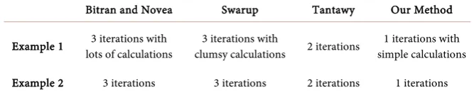
Table 1. Results of existing and our methods for Example 1 and Example 2.
Bitran and Novea Swarup Tantawy Our Method
Example 1 lots of calculations 3 iterations with clumsy calculations 3 iterations with 2 iterations simple calculations 1 iterations with
Example 2 3 iterations 3 iterations 2 iterations 1 iterations
Now different methods can be compared with our method and all the me-thods give the same results for Example 1 and Example 2. Table 1 shows the re-sults of number of iterations that are required for our method and the existing methods for these Examples.
6. Comparison
In this Section, we find that our method is better than any other available me-thod. The reason can be given as follows:
Any type of LFP problem can be solved by this method.
The LFP problem can be transformed into LP problem easily with initial guess.
In this method, problems are solved by algebraically with duality concept. So that it’s computational steps are so easy from other methods.
The final result converges quickly in this method.
In some cases of numerator and denominator, other existing methods are failed but our method is able to solve any kind of problem easily.
7. Conclusion
In this paper, we give an approach for solving linear fractional programming problems. The proposed method differs from the earlier methods as it is based upon solving the problem algebraically using the concept of duality. This me-thod does not depend on the simplex type meme-thod which searches along the boundary from one feasible vertex to an adjacent vertex until the optimal solu-tion is found. In some certain problems, the number of vertices is quite large, hence the simplex method would be prohibitively expensive in computer time if any substantial fraction of the vertices had to be evaluated. But our proposed method appears simple to solve any linear fractional programming problem of any size.
References
[1] Charnes, A. and Cooper, W.W. (1962) Programming with Fractional Functions. Naval Research Logistic Quarterly, 9, 181-186.
https://doi.org/10.1002/nav.3800090303
[2] Bitran, G.R. and Novaes, A.G. (1973) Linear Programming with a Fractional Objec-tive Functions. Operations Research, 21, 22-29. https://doi.org/10.1287/opre.21.1.22 [3] Bitran, G.R. and Magnanti, T.L. (1976) Duality and Sensitivity Analysis with
[4] Sing, H.C. (1981) Optimality Condition in Fractional Programming. Journal of Op-timization Theory and Applications, 33, 287-294.
https://doi.org/10.1007/BF00935552
[5] Swarup, K. (1964) Linear Fractional Programming. Operation Research, 13, 1029- 1036. https://doi.org/10.1287/opre.13.6.1029
[6] Tantawy, S.F. (2008) A New Procedure for Solving Linear Fractional Programming Problems. Mathematical and Computer Modelling, 48, 969-973.
https://doi.org/10.1016/j.mcm.2007.12.007
[7] Tantawy, S.F. (2014) A New Concept of Duality for Linear Fractional Programming Problems. International Journal of Engineering and Innovative Technology, 3, 147- 149.
[8] Effati, S. and Pakdaman, M. (2012) Solving the Interval-Valued Linear Fractional Programming Problem. American Journal of Computational Mathematics, 5, 51-55. https://doi.org/10.4236/ajcm.2012.21006
[9] Pramanik, S., Dey, P.P. and Giri, B.C. (2011) Multi-Objective Linear Plus Linear Fractional Programming Problem Based on Taylor Series Approximation. Interna-tional Journal of Computer Applications, 32, 61-68.
[10] Tantawy, S.F. (2008) An Iterative Method for Solving Linear Fractional Program-ming (LFP) Problem with Sensitivity Analysis. Mathematical and Computational Mathematics, 13, 147-151.
[11] Tantawy, S.F. and Sallam, R.H. (2013) A New Method for Solving Linear Fractional Programming Problems. International Journal of Recent Scientific Research, 4, 623- 625.
Submit or recommend next manuscript to SCIRP and we will provide best service for you:
Accepting pre-submission inquiries through Email, Facebook, LinkedIn, Twitter, etc. A wide selection of journals (inclusive of 9 subjects, more than 200 journals)
Providing 24-hour high-quality service User-friendly online submission system Fair and swift peer-review system
Efficient typesetting and proofreading procedure
Display of the result of downloads and visits, as well as the number of cited articles Maximum dissemination of your research work