Munich Personal RePEc Archive
Network security
Larson, Nathan
University of Virginia
11 August 2011
Online at
https://mpra.ub.uni-muenchen.de/32822/
Network Security
Nathan Larson
Department of Economics
University of Virginia
[email protected]
August 11, 2011
Abstract
In a variety of settings, some payoff-relevant item spreads along a network of connected individuals. In some cases, the item will benefit those who receive it (for example, a music download, a stock tip, news about a new research funding source, etc.) while in other cases the impact may be negative (for example, viruses, both biological and electronic,financial contagion, and so on). Often, good and bad items may propagate along the same networks, so individuals must weigh the costs and benefits of being more or less connected to the network. The situation becomes more complicated (and more interesting) if individuals can also put effort into security, where security can be thought of as a screening technology that allows an individual to keep getting the benefits of network connectivity while blocking out the bad items. Drawing on the network literatures in economics, epidemiology, and applied math, we formulate a model of network security that can be used to study individual incentives to expand and secure networks and characterize properties of a symmetric equilibrium.
1
Introduction
Being connected can be both a blessing and a curse. In this paper we build a model of network formation and security in which there are both benefits and risks to being highly connected to other agents. Our focus is on the role of the network in spreading non-rival goods (or bads) that are essentially costless to reproduce and transmit, such as news or viruses. While an agent joins the network to try to expose herself to any goods — denoted “tips” — that arise, as a consequence of join-ing she may also be exposed to bads, which we generically call “viruses.” Because tips and viruses exploit the same network structure to spread, both positive and negative network externalities will arise from the fact that individual decisions about connections affect others’ exposure. We assume that individuals can take costly actions that limit the spread of viruses without hindering tips; we call this security provision. This introduces a third externality, since an individual who blocks a virus benefits all of the downstream agents that she would have otherwise infected. We study the micro (individual connection and security choices) and macro (penetration rates of tips and viruses) properties of equilibrium in a large anonymous economy. To model “large and anonymous,” we adopt a random graph approach to network formation.
to benefit from word of mouth information, these physical connections between people also form a vector for the spread of disease. People can mitigate disease spread through individual effort, such as hand-washing and vaccinations. Alternatively, the virus may be electronic. Computer users benefit from information spread by various types of networks (such as email, file-sharing, or social media), but undesirable items such as viruses or spam can piggyback on these networks as well. A user can protect herself (and others) by screening email, installing anti-virus software, and so forth. In both cases, it is most natural to think of the tip as information, which by its nature is easily reproduced and transmitted, and often non-rival. Both biological and computer viruses share these characteristics.
In some other settings, our model may provide useful intuition about tradeoffs between openness and security, even when the application does not precisely match the model assumptions. For example, in financial markets, both valuable and worthless information circulate, and acting on worthless information can be costly. In this case, one might think of security as undertaking due diligence before acting on a rumor and passing it on to other people. Here, the connection to our model is not tight for various reasons, but some of the incentives and externalities will be similar.1 At an even broader, more heuristic level, there is a tension between the general benefits of an open, interconnected society (such as ease of communication, electronic banking, and so forth) and the threat that those very interconnections could make the society more vulnerable to attack, by terrorists or other malefactors.
As a general template for thinking about issues of connectivity and security in a large anonymous economy, suppose that we give an agent two choice variables: z, which will be some measure of his connection intensity or how actively he participates in the network, andf (for firewall), which will be some measure of his efforts toward avoiding the threats it poses. Suppose that a is some aggregate variable that summarizes the “good connectivity” of the network — that is, how well it spreads tips — and b is an aggregate variable that summarizes “bad connectivity” — that is, how prevalent viruses are. To make this the barest of reduced form models, we would need (inter alia) two elements: a payoff function for agents, and a general equilibrium mechanism specifying how individual choices(z, f) aggregate,via some network structure, to get the summary parametersa
and b. A simple payofffunction could have the form
Benef it(z, f;a)−Harm(z, f;b)−Cost(z, f) (1)
whereC(z, f)reflects some direct costs of connections and security, and thefirst two terms capture the benefits earned and harms suffered from exposure to the network. At this stage, a modeler
might impose some desired form of network externalities, perhaps in the form of constraints on the cross partial derivatives of the benefit and harm functions. One motive of the paper is to provide primitive foundations for this reduced form model. We will introduce an explicit network formation process, derive aggregate parameters aandb, and show that individual payoffs take the
form of (1). Furthermore, by micro-founding the benefit and harm functions, we will be able to derive the structure of network externalities rather than impose it. In linking what might be called the structural and reduced form models, we aim to address the relatively common complaint that
1Two important distinctions are that
network theory is impractical for applied work because it relies too delicately on fine details of network structure that are rarely observed in data. In our model, the properties of the network that matter for incentives can be characterized very compactly.
The model is simplest to describe by beginning in the middle. Suppose that agents’ connectivity and security choices have generated a network, modeled by a graph in which agents are nodes and connections between them are links. Certain links arefirewalled in one or perhaps both directions; this means that a virus cannot travel along this link in the firewalled direction. The following completely exogenous events happen next. First, Nature creates a single tip or virus and endows it on a randomly chosen agent (the “Origin”). Then, if it is a tip, it spreads to every agent who is linked either directly or indirectly to the Origin. Alternatively, if Nature endows a virus, it spreads in the same way, but only along links that have not been firewalled. Finally, all agents who have been exposed receive a common payoff(positive for a tip, negative for a virus); there is no decay or discounting. The exogenous generation and transmission of tips and viruses is intentionally quite stylized, as the focus of this paper is elsewhere.
All of the strategic decisions happen one stage earlier. Although agents will act simultane-ously, in spirit we wish to capture the idea that an agent faces a large, anonymous population of potential contacts, with only weak information about how they are interconnected or about who is particularly vigilant. To capture this, we use a random graph model of network formation. Agents simultaneously choose link intensities and security efforts(z, f). The link intensity could be thought of as undirected effort devoted toward forming contacts, which pays offwith a stochastic number of links. A higher security level means that more of these links will befirewalled, although this too has a random component. Although agents are constrained by the technology of network formation, they are fully rational: in a Nash equilibrium,zandf are chosen with respect to correct expectations about others’ strategies, and what they imply about the aggregate properties of the network.
While the model is formulated with a finite number of agents, all of the analysis will focus on the large population limit where we can exploit sharp limiting results for random graphs. There is one other feature of the model that serves a technical purpose in this paper but could be interesting to study in its own right. In addition to the strategic agents, there is one large, nonstrategic agent called the hub. At the network formation stage, separately from the strategic choicez, every agent also forms a link to the hub with a small exogenous probability. Tips and viruses pass through the hub just as they do through other agents. All of our analysis will focus on the decentralized limit in which the “size” of the hub (that is, the probability of linking to it) is taken to zero. The purpose of introducing this central institution only to take it away is somewhat analogous to seeding a rain cloud or providing a dust particle as a nucleus for a snowflake. The relevant limiting properties of the network as the hub vanishes are no different than they would have been had it never existed at all, but they are substantially easier to characterize rigorously. For an economic interpretation, it makes the most sense to think of an institution, such as a government or a healthcare system, or a forum where clusters of people can gather, such as a website or a club. However, since the role of the hub will be vanishing and mechanical in this paper, we will not push these interpretations too far.
same is true for the fraction of the population infected by a virus. These fractions, which we call
a and b, turn out to be the key aggregate variables for understanding individual incentives. The mathematical form of a is well known in the graph theory literature for the case when all link intensities are symmetric, but equilibrium analysis demands that we consider asymmetric cases as well (either because the equilibrium is asymmetric or to evaluate deviations from a symmetric equilibrium). Similar demands arise for b. A modest technical contribution of the paper is to provide rigorous derivations for these cases (Propositions 1 and 2).
We confine our equilibrium analysis to symmetric equilibria. The interaction of three externali-ties — positive and negative network externaliexternali-ties, and the public good problem of security provision — generates a rich and nuanced spectrum of outcomes. One feature that contributes to this richness is the fact that there are increasing returns to security. This is due to a type offinger-in-the-dyke effect: the marginal benefit from protecting a single link is small since one is likely to be infected anyway through other channels. By favoring all-or-nothing security investments, this works against symmetry, as it is not stable for everyone in the network to be fully secure or completely lax.2 However, symmetric equilibria do exist when the cost of security is sufficiently convex, and we study comparative statics for cases in which those costs are also independent of the number of links protected.3 When security is relatively expensive, equilibria fall into two general classes. If the
severity of threats is low (that is, if viruses are rare or the payoffpenalty from exposure is mild),
then a Wild West scenario prevails: people form links profusely, pay lip service to security, and both the tip exposure rate a and the infection rate b are high. This reverses if threat severity is high: people cut links drastically (as a substitute for securing them), the network shrinks, and both
a and b are small. Moreover, in the latter case, downward shifts in security costs (due perhaps to new technology or subsidy policies) will unambiguously make infection rates worse (higher b) before they eventually improve. The reason is that the lower security costs make it attractive to form more links, and the aggregate effect of a denser network on virus transmission swamps the increase in security. If such a change were to result from a policy initiative like a subsidy, it would be easy to jump to a judgement the policy had failed. We show that if total welfare is the yardstick (and not infection ratesper se), then this judgement would be mistaken, as total welfare, including the benefits from a denser network, unambiguously rises with such a change.
Next, we put equilibrium networks through a stress test by taking the severity of threats to infinity. A network isresilient if it does not collapse under this process — that is, ifaand individual payoffs remain strictly positive. We show that loosely speaking, a network will be resilient if and only if agents can obtain at least a small amount of security for free. (More precisely, thefirst three derivatives of the cost function must vanish atf = 0.)
The issues addressed in our model have received attention across a broad spectrum of acad-emicfields and in various applied settings, as one might expect, given the diverse area of topics to which network flows are germane. In the epidemiology literature, models of disease spread tradi-tionally have employed strong assumptions about how populations mix that allow the analyst to avoid modeling networks explicitly. Instead, these assumptions permit disease transmission to be characterized in terms of systems of differential equations. However, as more recent work by Mark
2
We study the case in which equilibria must be asymmetric in companion work.
3Thus these cases are closer to a
Newman and various coauthors (notably Newman et al. 2001) has illustrated, the consequences of assuming away the network structure of disease transmission are not innocuous. This more recent work takes a graph theoretic approach similar to ours. It is worth highlighting three important differences between these papers and ours. First, in considering disease epidemics, Newman (2002) employs a more detailed model that adheres more closely than we do to the specific features of a disease outbreak. In contrast, to make the novel features of our model as clear as possible, we have kept it simple and avoided wedding it too closely to any specific application.
More importantly, the methodology of Newman et al. (2001) and most of the closely related literature involves using ingenious but non-rigorous generating function arguments establish claims. To apply this approach, one must be willing to assume properties for the random graph, such as zero probabilities for some rare events, or independence for weakly correlated events, that are not strictly true for a finite graph but that one plausibly expects to hold in the limit. Vega-Redondo (2007) and Jackson (2008) provide accessible treatments of this approach in an economics context. On the other hand, when link intensities are asymmetric, rigorous proofs of aggregate network properties by probabilists, as in Molloy and Reed (1995) and (1998) and Chung and Lu (2002), can be quite lengthy. Since for an economist, these aggregate network properties are in the service of an economic insight but are not the end in themselves, a modeling strategy that admits parsimonious but rigorous proofs is attractive. Our device of an infinitesimal hub accomplishes this (although the proofs are still not as short as one might like).4
Finally, and most importantly for economists, existing network models based on a random graph generating function approach almost universally treat individuals’ behavior as exogenous. Our main innovation is to take individual incentives seriously in the context of an equilibrium model.
Within economics, there has been a steadily growing interest in interactions on networks, with seminal treatments of network formation by Jackson and Wolinsky (1996) and Bala and Goyal (2000), among others; for book length treatments, see Goyal (2007), Jackson (2008), and Vega-Redondo (2007). A number of recent papers including Goyal and Vigier (2011), Hoyer and De Jaegher (2010) and Kovenock and Roberson (2010) study issues of security and reliability of a network under threat, but the focus in these papers is almost perfectly orthogonal to ours. They look at situations in which a centralized network designer (or designers) chooses a detailed network structure with an eye toward foiling the attack of a hostile strategic agent who is well informed about the structure of the network. Explicitly modeling the behavior of threats is an important element that we set aside to focus on other issues. The nature of threats differs somewhat in our setting, as our viruses operate not by disrupting the network but by hijacking it. But more importantly, our focus on the individual incentives of small, decentralized agents who are not able to act on the basis of detailed information about the network structure represents the polar opposite of a command and control design problem.
In the next section, we introduce the model for a finite number of agents and a positive hub size; then we discuss the limits as the number of agents grows and the hub shrinks. Section 3 derives the aggregate network properties of interest and uses them to derive expressions for agents’ payoffs. An impatient reader who is willing to take the results of Propositions 1 and 2 on faith may want to skip ahead to Section 3.2, or even Section 4. Section 4 presents equilibrium conditions and
studies the properties of symmetric equilibria. Section 5 concludes with a discussion of limitations and extensions.
2
Model
2.1
Networks and Items
An nh−economy consists of n small strategic agents, indexed {0,1,2, ..., n−1}, and one large, nonstrategic player called the hub (H). The term h refers to the size of the hub and will be discussed later. We call the limit of an nh−economy as n → ∞ a large h−economy, or just an
h−economy. If we additionally let the influence of the hub vanish (in a way to be specified later), we call the result alarge decentralized economy. Our results will focus mainly on large decentralized economies.
The small agents make strategic choices that influence the creation of a network, which we model as an undirected random graph in which agents are vertices and links between agents are edges. Formally, letting In = H ∪{0,1,2, ..., n−1}, a network for an n−economy is a function
G :In2 →{0,1}, whereG(i, j) = 1 if and only if there is a link between agentsiandj. Because the
graph is undirected, we haveG(i, j) =G(j, i)for alliandj. Self-links (G(i, i) = 1) are not ruled out
per se, but they will not of any particular interest in what follows. Several notions of connectivity
in G will be important. Define the tth order neighbors of i by N1
G(i) ={j∈In| G(i, j) = 1} and
Nt
G(i) = ©
j ∈In| G(i0, j) = 1 for somei0∈NGt−1(i)
ª
. We say that i and j communicate in G if there is a sequence of links that connects them. Mathematically, we write j ∈ NG(i), where
NG(i) = {i}∪¡S∞t=1NGt(i) ¢
; note that j ∈ NG(i) and i ∈ NG(j) are equivalent. From time to
time, if there is no ambiguity aboutG, we may use the notationi←→1 j to mean that iandj are first order neighbors, and i←→ j to mean that they communicate. A component of the network is a maximal subsetC ⊆Insuch that all of the agents inC communicate with each other; that is,
i←→j for all i, j∈C, and i=kfor all i∈C and k∈In\C.
Any undirected graph can be reinterpreted as a directed graph in which each undirected link
i←→1 jis represented by a pair of directed edges fromitoj, writteni7→1j, and fromjtoi. Given
a network G, an unsecured subnetwork Gf is a directed subgraph of G, formed from G’s directed
counterpart by deleting a subset of the edges. Formally, let Gf be a function Gf : I2
n → {0,1},
where we do not requireGf(i, j) =Gf(j, i), andGf(i, j) = 1(equivalently, i7−→
1 j) is interpreted
to mean that there is a directed edge from i to j. Then Gf is an unsecured subnetwork of G if
Gf ≤ G. For reasons that will be clear shortly, we say that i directly infects j if i7−→
1 j, andi
infects j (written i 7−→ j) if there is some chain of agents {k1, k2, ...} and edges i 7−→1 k1 7−→1
k2 7−→1 ... 7−→1 j leading from i to j. Define an agent’s upstream and downstream neighbors:
NGU pf (i) ={j∈In|j7−→i}∪{i}and NGDownf (i) ={j∈In|i7−→j}∪{i}.5 In general, these sets
will not coincide, but note thatj∈NGU pf (i) if and only if i∈N Down
Gf (j).
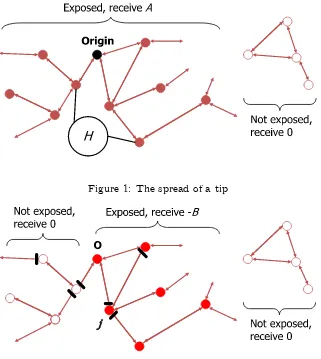
The role of the network in our model is to transmititems. Items come in twoflavors, desirable and undesirable, which we label as tips and viruses respectively. Items are generated and spread in a mechanical way: after the network is formed, one randomly chosen agent is endowed with one item, which is a tip with probability λand a virus with probability1−λ. This agent is called the
5
Figure 1: The spread of a tip
Figure 2: The spread of a virus. Firewalls indicated by black bars. While agent j firewalls her direct link to O, she is still infected indirectly.
origin, and without loss of generality, we take him to be agent 0.6 If the item is a tip, it spreads (costlessly and with no degradation in quality) along the links in G. On the other hand, a virus spreads only to agents who are downstream of the origin. An agent who is exposed to the item (including the origin) receives a payoff of A > 0 if it is a tip, or −B (where B > 0) if it is a virus, while an agent who does not receive the item gets a payoff of zero. Multiple exposure has no additional effect; the payoff of A or −B is realized at most once by each agent. Thus, agent
i receives A if there is a tip and i ∈ NG(0), −B if there is a virus and i∈ NGDownf (0), and zero
otherwise.
2.2
Network Formation and Security
An agent imakes two strategic decisions, denoted zi ∈ [0,∞) and fi ∈[0,1]. The first one is her
link intensityzi, this determines the mean number of links she will form to other small agents. The
networkG is a random graph in which a link betweeniandjappears with probability proportional tozizj. The exception is the hub: each agent forms a link to the hub with exogenous probability
6
h. We will sometimes refer to h as the size of the hub. The other decision is a security level fi:
this reflects effort to screen out incoming viruses. If i←→1j inG, theni blocks an infection from
j (j 67−→1 i in Gf) with probabilityfi.Thus, for a given networkG, positive security levels fi > 0
create a wedge ensuring that viruses do not spread as widely as tips. Timing is as follows: all agents simultaneously choose zi and fi; then graphs G and Gf are generated; and finally, a single item is
generated, endowed on agent 0, and spreads over the network as described above. Remember that agent 0 does not know that he is the origin; labeling him this way is just for our convenience. Now we turn to a more precise statement of how the random graphs G and Gf are formed.
Let (z,f) be a strategy profile for the strategic agents, where z = (z0, z1, ..., zn−1) and f =
(f0, f1, ..., fn−1). On occasion we may write (zn,fn) where it is important to emphasize the size
of the economy. Conditional on (z,f), generate the following collections of independent, binary zero-one Bernoulli random variables:
ζij for all i, j ∈ In\H such that i≤j
ηi for all i ∈ In\H
φij for all i ∈ In and j∈In\H
The first set of n(n2+1) random variables determines whether there is a link between small agents
i and j in G. Whenever i < j, define a mirror image variable ζji equal to the realization of ζij. Then set G(i, j) = ζij for all i and j in In\H. The probability that a link exists between i and
j is assumed to be Pr¡ζij= 1¢=pij = znizz¯j, where z¯= n1Pmn−=01 zm is the average link intensity.7
Notice that agenti’s expected number of links to other small agents is
E ⎛
⎝ X
j∈In\H ζij
⎞ ⎠=zi
P
j∈In\Hzj
nz¯ =zi
so it is reasonable to think ofzi as agenti’s choice of an expected number of connections.
The next set ofnrandom variables determines whether there is a link between each small agent and the hub: we setG(i, H) =G(H, i) =ηi for alli∈In\H. The probability of linking to the hub
isPr (ηi= 1) =h, independently across agents, and regardless of the strategy profile.
The final set of n(n+ 1) random variables determines whether there is a firewall that blocks the transmission of a virus fromitoj. Thesefirewalls determine the construction of the unsecured subnetwork Gf relative toG:
Gf(i, j) =
⎧ ⎪ ⎨ ⎪ ⎩
¡
1−φij
¢
ζij =
¡
1−φij
¢
G(i, j) ifi, j∈In\H
¡
1−φHj¢ηj =¡1−φHj¢G(H, j) ifi=H, j∈In\H
ηi=G(i, H) ifj=H
As the definition above indicates, thefirewall variable φij only becomes relevant in the event that Ghas a link betweeniandj: in this case we construct the subnetworkGf by removing the directed
edge i 7−→1 j if φij = 1, and retaining it if φij = 0. Note that φij and φji are two different,
independent random variables: j being protected against infection by iis unrelated to whether j
7To ensure thatPr¡ζ
ij= 1
¢
≤1, we do need to impose maxIn\H(zi) 2
can infect i. Small agents protect their links with the hub in the same way that they protect all of their other links. By assumption, the hub puts up no defenses; any virus that reaches it passes through unhindered. The probability of blocking a virus depends entirely on the security level of the receiving agent: Pr¡φij= 1¢=fj, independently acrossi∈In, for all j∈In\H.
A few remarks about this security technology may be helpful at this point. First, by choosing
fj = 1, an agent can guarantee that she screens items perfectly. For any fj < 1, her security
will make mistakes with positive probability, and by assumption, these mistakes are on the side of excessive laxness (viruses sneaking through) rather than excessive vigilance (tips being accidentally blocked). We make no defense for this assumption, other than that it simplifies the analysis — expanding the analysis to incorporate both types of mistake would be a natural extension. It is expositionally convenient but inessential to assume that thefirewall variables are realized simulta-neously before the item is generated. We could alternatively assume thatφij is not realized unless a virus actually arrives at j from i, in which case the security technology succeeds in blocking it with probability fi — nothing in the model would change under this reinterpretation.8
To illustrate what it means for the random variables φij to be independent across i, consider a concrete example of a computer virus. In one scenario, suppose there is a universe V consisting of V = |V| different viruses, one of which is dropped randomly on agent 0. Suppose a security technology of quality f is a software package that can recognize and block f V of the viruses in V. In this case, we might think of φij and φi0j as perfectly correlated: if (with probability fj)
the virus is one that her antivirus software recognizes, then j is protected along all of her links; otherwise she is not protected at all. In an alternative scenario, suppose that blocking an incoming virus requires different techniques depending on whether the connection is an email attachment, a transfer of packets with a web site, an instant message conversation, a Skype phone call, or some other communication channel. If jtends to communicate on different channels with different neighbors and antivirus software does not protect all of these channels equally well, then we would not expectφij andφi0j to be perfectly correlated. For now, we focus on the latter type of situation. We reiterate that an agent icommits to (and pays for, as we shall see momentarily) a security levelfi at the same time that she chooses how connectedzi to be. Thus she chooses ‘under a veil
of ignorance’ in two senses. First, she does not see her realized number of links before choosing
fi; if she did, she would presumably want to adjust the diligence of her protection depending on
whether she is more or less connected than she expected to be. Second, she cannot focus her security efforts toward some neighbors more than others — all of her links have the same chance
fi of being protected. While this is surely too extreme, we are constrained by tractability, and in
keeping with the ethos of the paper, we err in the direction of making agents too ignorant rather than too informed.
2.3
Payo
ff
s and Equilibrium De
fi
nition
We are now in a position to formally define payoffs and equilibrium. As above, let (z,f) be a strategy profile. A strategy profile in which agent iplays according to some (zi, fi) and the other
agents play according to (z,f) is written ¡(zi, fi) ; (z,f)−i
¢
. Agenti’s payoffis
8This is because the strategic choices z
i and fi precede the realization of any of the random variables, so it is
πi
¡
(zi, fi) ; (z,f)−i
¢
= λA Pr
ζ,η,φ(i∈NG(0) |zi,z−i)
−(1−λ)B Pr
ζ,η,φ
¡
i∈NGDownf (0)|(zi, fi),(z,f)−i
¢
−C(zi, fi)
The subscript(ζ,η,φ), which we will suppress from now on, is a reminder that these probabilities are taken over realizations of the link and firewall random variables. Because the frequency λ of tips never appears separately from their magnitudeA, we will absorbλintoA. Similarly, we absorb 1−λintoB, rewritingi’s payoffas
πi¡(zi, fi) ; (z,f)−i¢=APr (i∈NG(0)|zi,z−i)−BPr¡i∈NGDownf (0)|(zi, fi),(z,f)−i¢−C(zi, fi)
The final term represents the explicit costs of choosing connectivity zi and security fi. For the
most part, we will assume that forming links is not costly per se, but zi still appears in the cost
function because the cost of security may rise with the number of links secured. If the cost of attaining security level f rises linearly with the number of links, then we have C(z, f) = zc(f); we refer to this as the constant M Clink case. At the other extreme, if C(z, f) = c(f), then the
cost of protecting z links at level f does not depend on z. This is referred to as thezero M Clink
case. Which version of costs is appropriate (if either) will depend on the specific application. For example, the nuisance cost of handwashing might be expected to scale up withz, whereas a single
flu shot could provide protection against any number of exposures to a particular strain of influenza. We will often impose the following set of regularity conditions on c(f).
A1 The function c : [0,1] → R+ is continuously differentiable, strictly increasing and strictly
convex on(0,1], and satisfiesc(0) = 0,c0(0) = 0, andlimf→1c0(f)≥B.
While convexity and the other conditions in A1are introduced with an eye toward giving the individual’s security decision a unique, interior optimum, they do not guarantee this — there are parameter regions, and cost functions satisfying A1, for which equilibria with symmetric interior security levels do not exist. The reason is that the returns to security will also turn out to be convex.
These payofffunctions extend naturally to largeh−economies and large decentralized economies. Now let z andf be infinite sequences, with zn (fn) the truncation ofz (f) to itsfirst nterms. We interpret the pair of truncated sequences (zn,fn) as a strategy profile in a nh-economy. In the sequel, when we need to separate out the strategic decision (zi, fi) of one agenti with respect to
anticipated behavior(z,f)−i by the other agents, we will often takei= 1without loss of generality. In a large decentralized economy, agent 1’s payoff from playing (z, f) when the other agents play according to (z,f)−1 is defined to be
π1¡(z, f) ; (z,f)−1¢ = lim
h→0nlim→∞π1
¡
(z, f) ; (zn,fn)−1¢ = AA(z;z−1)−BB¡(z, f) ; (z,f)−1
¢
where
A(z;z−1) = lim
h→0nlim→∞Pr
¡
1∈NG(0) |z,zn−1 ¢
B¡(z, f) ; (z,f)−1¢ = lim
h→0nlim→∞Pr
¡
1∈NGDownf (0)|(z, f),(zn,fn)−1
¢
Of course, this payoff is only well defined if the relevant limits exist; later we will show that they do for the cases that are of interest.
The reason for the order of limits, although technical, is important enough to mention. Our modeling owes a heavy debt to the random graph literature, where the typical approach is to study the connectivity of a finite hubless network as n → ∞, in effect reversing our order of limits. In that literature, there is a substantial gap between what is ‘known’ to be true based on clever, semi-rigorous arguments, and what has actually been formally proved. One well established result is that a sufficiently connected large random graph has (with probability tending to one asn→ ∞) a single large O(n) component, called the giant component, while all other components are small (O(logn)or smaller). In our model, the hub acts as a seed for this giant component. This simplifies proofs tremendously by allowing us to break down compound events involving the connectivity ofi
and j into simpler events about how each of them is connected toH. As far as we are able to tell, our results would be identical if the order of limits were reversed, but the proofs would be much more cumbersome.
Now we can define an equilibrium for a large decentralized economy.
Definition 1 A large decentralized economy (LDE) equilibrium is a strategy profile (z∗,f∗) such that
i) πi¡(zi, fi) ; (z∗,f∗)−i¢ is well defined for all (zi, fi) ∈[0,∞)×[0,1], for all i ∈ {0,1,2, ...},
and
ii) (zi∗, fi∗) maximizes πi
¡
(zi, fi) ; (z∗,f∗)−i
¢
for all i∈{0,1,2, ...}.
Notice that we define our equilibrium directly in terms of the limiting payoffs, not as the limit
ofnh-economy equilibria — one should keep this in mind when thinking about the LDE results as an approximation of behavior in a largefinite economy.9 One can think of a symmetric strategy profile, in the natural way, as a profile in which every agent uses the same strategy (z, f). Asymmetric profiles and mixed profiles over a finite set of supporting strategies can be thought of informally in terms of the limiting population shares of each strategy as n goes to infinity; we will be more precise about this later. For strategy profiles like these, existence of the limiting payoff functions is not an issue. For most of the paper, we will focus on symmetric equilibria; the next section is devoted to characterizing the limit payoffs for this case.
3
Limiting Properties of
G
and
G
f: the Symmetric Case
In this section, we derive explicit expressions for the limiting probabilitiesA(˜z;z−1)andB ³³
˜
z,f˜´; (z,f)−1´ when the strategy profile(z,f)−1specifies that all agents other than agent 1 play the same strategy
9To be precise, the
(z, f). As a side note, one could imagine a different modeling approach in whichAandBare taken as the primitives that describe theflows of benefits and harms on a network. One secondary goal of the analysis in this section is to shed light on some of the features one might want to impose on Aand Bif they were taken as primitives of a network model. The analysis starts with the simpler case of tips (A). In the course of informally deriving A (proofs are in the appendix), we provide a thumbnail sketch of some of the limiting properties of a large network. In what follows, the phrase “with probability tending to 1 as n→ ∞” is a common modifier, so it is useful to have shorthand. We will write this as (pt1).
3.1
Characterization of the Spread of Tips and Viruses
Proposition 1 Suppose that z is the symmetric limit strategy profile with every term equal to z. Then for all z˜,
A(˜z;z−1) = (
0 if z≤1
a¡1−e−az˜¢ if z >1
where a is the unique positive solution to
1−a=e−az . (2)
We start by developing some intuition for Proposition 1 along with some of the machinery used in the proof; the formal proof is in the appendix. The basic idea is the following. First we show that it is without loss of generality (pt1) to assume that if agents 0 and 1 communicate, they do so through the hub. Then to compute the probability that, say, agent 0 communicates with H, we couple the true enumeration of extended neighbors of 0 (byfirst order neighbors, then second order neighbors, and so forth) to a related branching process. The branching process overestimates the number of neighbors by not treating a doubling back to a previously visited agent as a dead end. The probability that the branching process dies out before any of its members connect toH is easy to compute. While this underestimates the probability that the true extended neighborhood fails to connect toH, we can show that the difference vanishes asn→ ∞. The reason is that conditional on failing to connect to H, the branching process must have died out at a small size relative to
n (pt1), in which case it is very likely (pt1) that the branching process and the true enumeration never diverged (due to no double-backs). Below, we provide a more complete discussion of some of these steps.
It helps to have a term for the set of small agents who communicate with i(includingiherself), without using any links to or fromH. Define
Si =i∪{j∈In\H|iand j communicate along at least one path that does not include H}
Next, notice that the eventi=H(ifails to connect to the hub) is equivalent to the event that for all agents j ∈Si, the random variables ηj have realization zero. We will get considerable mileage
out of the fact that (for fixed h) this event becomes very unlikely if we condition on |Si| being
large: an agent who has many small neighbors is very likely to be connected to the hub as well. In what follows, Si large will often be taken to mean|Si|>logn, while we may say that Si is small if
Next observe that the event that agents 0 and 1 communicate can happen in one of two disjoint ways. First, they may connect through the hub: 0 ↔ H and 1 ↔ H implies 0 ↔ 1.10 Or, they might be connected with each other despite the fact that neither is connected to H; this is the event1↔0 ∩1=H∩0=H. Thefirst step of the proof is to show that this second case is very unlikely. The logic is that if agent0fails to connect toH, then by the argument above,S0 must be
small. The same is true for agent 1 and S1. But absent a connection to the hub, S0 and S1 must
intersect if we are to have 0↔1, and the chance of this intersection vanishes ifS0 and S1 are both
small.
Thus, to determine the chance that 0 and 1 communicate, it suffices to focus on thefirst case: the probability that agents 0 and 1 both communicate with the hub. The next step is to show that the events 0 ↔ H and 1 ↔ H are approximately independent, so A(˜z;z−1) reduces to the
product of their (limiting) probabilities. It is easier to grasp the intuition of this independence for the complementary events 0=H and 1=H. These events can only occur ifS0 and S1 are both
small, but in this case, they cannot have much influence on each other. In summary, it suffices to characterize the probabilitiesPrnh¡0=H|z,˜ zn−1
¢
andPrnh¡1=H|z,˜ zn−1 ¢
. To characterize the probability of0=H, we introduce a thought experiment. Let each small agent
in{0, ..., n−1}represent a ‘type,’ and suppose that we can generate arbitrarily many distinct
indi-viduals of each type. We grow a population of these indiindi-viduals according to the following branching process. Let Wˆt be the set of individuals alive at generationt, and letRˆt be the set of individuals
who were previously alive. The individuals inWˆthave children, according to probabilities described
below, and then die; thus we have Rˆt+1 = ˆRt∪Wˆt. An individual of type i has either zero or one
child of each type, where the probability that she has a child of type j is pij. (Thus the total
number of progeny for this individual is the sum of nBernoulli random variables.) These random variables are independent across individuals. The setWˆt+1 is defined to be the set of all children of
individuals inWˆt. In general, Wˆt and Rˆt may contain many distinct individuals of the same type.
The process itself dies out ifWˆT is empty, for some T, in which case Rˆt= ˆRT for all t≥T.
If we initialize this process with Rˆ0 = ∅ and Wˆ0 containing exactly one individual of type 0,
then we can associateWˆ1 with agent 0’s first order small neighbors. Furthermore, as long as all of
the individuals inRˆt have different types, we can associateRˆt with the subset of agents in S0 who
are reachable withintlinks of agent 0. However at some point Wˆt may include a child whose type
already appears inRˆt. From the standpoint of enumerating the agents inS0, we should ignore this
child, and her progeny, to avoid overcounting. Instead, the process counts her and treats her as an independent source of population growth. For this reason,P∞t=0
¯ ¯ ¯Wˆt
¯ ¯
¯ is larger than|S0|. However,
in the event that S0 turns out to be small, it is very likely that the branching process does not
generate any of these duplicates, and therefore enumeratesS0 exactly.
Next, endow each individual inWˆt(for allt∈{0,1,2, ...}) with an i.i.d. binary random variable
that succeeds or fails with probability h or1−h. By analogy with the true model, call a success a connection to the hub. Let Yˆnh
0 be the probability that these random variables fail for every
individual in S∞t=0Wˆt; since this comprises weakly more individuals than there are agents inS0,
we havePrnh¡0=H|z,˜ zn−1 ¢
≥Yˆnh
0 . Furthermore, the difference between these two probabilities
is small because 0 = H can only occur when S0 is small, in which case the branching process is
very likely to enumerate S0 correctly. Fortunately Yˆ0nh is straightforward to compute.
To simplify the computation, pool individuals of typesN\ {1}together as “normal” types, since their reproduction is governed by exactly the same probabilities, and refer to type 1 as the “deviant” type. A normal individual producesBin(n−1, p00)normal children andBin(1, p01)deviant ones,
whereas a deviant individual has Bin(n−1, p01) normal children and Bin(1, p11) deviant ones.
Let Eˆ0 be the event that no individual in the branching process beginning with a single normal
individual connects toH, soYˆnh
0 = Prnh
³
ˆ
E0
´
. LetEˆ1 be the corresponding event for a branching
process beginning with a single deviant individual, with Yˆnh
1 = Prnh
³
ˆ
E1
´
. Observe that Eˆ0
requires that (i) the initial individual does not connect to H, (ii) for each potential normal child, either this child does not exist, or she does exist, and event Eˆ0 holds for the independent process
beginning with her, and (iii) for each potential deviant child, either the child does not exist, or she does exist, and eventEˆ1 holds for the independent process beginning with her. These conditions are
all independent; (i) occurs with probability 1−h, (ii) occurs with probability³1−p00+p00Yˆ0nh ´
for each potential normal child, and (iii) occurs with probability³1−p01+p01Yˆ1nh ´
for the single potential deviant child. Thus we have
ˆ
Y0nh = (1−h)³1−p00+p00Yˆ0nh ´n−1³
1−p01+p01Yˆ1nh ´
(3)
By the same type of argument,Yˆnh
1 must satisfy
˜
Y1nh = (1−h)³1−p01+p01Yˆ0nh ´n−1³
1−p11+p11Yˆ1nh ´
(4)
Notice that we can write the expression forY˜nh
0 as(1−h) ³
1−n+zd³1−Yˆnh
0
´´n−1³
1−n+z˜d³1−Yˆnh
1 ´´
,
whered= z˜−zz. Taking limits, we have
ˆ
Y0h = lim
n→∞
ˆ
Y0nh= (1−h) lim
n→∞
µ
1− z
n+d
³
1−Yˆ0nh´
n−1
lim
n→∞
µ
1− z˜
n+d
³
1−Yˆ1nh´
= (1−h)³e−z(1−Yˆ0h)
´
(1)
which has a unique positive solution that lies in the interval (0,1). Mutatis mutandis, the result forYˆh
1 is similar; taking limits, we have
ˆ
Y1h= (1−h)e−z˜(1−Yˆ0h)
The expression in Proposition 1 follows by settinga= limh→0 ³
1−Yˆh
0 ´
.
The formal proof follows the lines of the argument above. Most of the effort involves proving the various claims about events that occur with vanishing probability as n grows large. Also, in order to compare the branching process to S0 rigorously, we must construct them on the same
or without the hub, any two agents have a vanishing chance of communicating unless they both happen to belong to the unique giant component. Since its size implies that H belongs to the giant component (pt1), statements like 0↔ H turn out to be a tractable shorthand for agent 0’s membership in the unique giant component.
Notice that if all agents (including agent 1) play z, the expected fraction of the population that benefits from a tip isa2 : with probability athe originating agent communicates with a non-negligible set of agents, in which case fractiona of the population is exposed to her tip. In a large decentralized economy,aremains at zero unless connectivity rises above the threshold levelz= 1. This is a particularly acute form of network effect: for an individual, there is no point in forming connections unless aggregate connectivity is great enough. Notice that this result smooths out in a largeh-economy. If we writeah = 1−Yˆ0h, then it is not hard to see thatah is positive and strictly increasing for allz.
Next we turn to the spread of viruses.
Proposition 2 Let ³³z,˜ f˜´; (z,f)−1´ be the strategy profile in which agent 1 plays ³z,˜ f˜´ and every other agent plays (z, f). Then for all ³z,˜ f˜´,
B³³z,˜ f˜´; (z,f)−1´=
(
0 if z(1−f)≤1
b³1−e−b(1−f˜)z˜´ if z(1−f)>1
where b is the unique positive solution to
1−b=e−b(1−f)z .
Notice that the probabilityB³³z,˜ f˜´; (z,f)−1´is exactly the expression that would result from substituting ‘effective’ link intensity ³1−f˜´z˜ for agent 1, or (1−f)z for the other agents, in place ofz˜orz in Proposition 1. The simplicity of this correspondence between G and Gf depends
somewhat on the symmetry of this strategy profile; for general strategy profiles, one cannot simply substitute(1−f)z forz to get appropriate expressions forGf.
The logic follows the previous proposition quite closely. By analogy with Si, define Siup to be
the set of agents who infecti by some path that does not include H. That is j ∈Siup if and only if j 7−→1 i or j 7−→1 k1 7−→1 ... 7−→1 km 7−→1 i for some path that does not include H. Define
Sidown to be the set of agents whomi infects along some path that does not include H. We claim that if there is no infecting path from agent 0 to agent 1 through the hub (0 7−→H 7−→ 1), then agent 0 does not infect agent 1 through any path (pt1). To see why this is true, suppose that 0 7−→ H 7−→ 1 fails because 0 does not infect H. This is only possible if 0 infects relatively few agents (Sdown
0 ≤logn), in which case the chance that agent 1 is among those infectees is small. A
similar argument applies if 07−→H 7−→ 1 fails because agent 1 is not infected byH. This means that we can focus on infections that go through H. Next, by an independence argument similar to Proposition 1 it suffices to study the probability 07−→ H and H 7−→ 1 one at a time. Finally, the complementary probabilities of067−→H and H67−→1 can be computed by a branching process approximation that is exact in the large nlimit.
infectees of agent 0, define ³Wˆdown t ,Rˆdownt
´
just as³Wˆt,Rˆt
´
except for one key change. As above, an individual of typeihas either zero or one child of each type, but the probability that she has a child of typejis now given bypij(1−fj), where earlier it was simplypij. The interpretation is that
we only count progeny when a link is formed (with probabilitypij) and that link is not blocked by
the downstream child (with probability1−fj). As earlier, designate individuals of typesN\ {1}as
normal and individuals of type 1 as deviants. Under³Wˆdown t ,Rˆdownt
´
, a normal individual produces
Bin(n−1, p00(1−f)) normal children and Bin ³
1, p01 ³
1−f˜´´ deviant ones, while a deviant individual producesBin(n−1, p01(1−f))normal children andBin
³
1, p11 ³
1−f˜´´deviant ones. Each of these individuals is endowed with a probability h chance of infecting H. LetYˆidown,nh be the probability that, in a branching process ³Wˆtdown,Rˆdownt
´
starting with a single individual of type i, no individual in the process infects H. By substituting the new reproduction rates into equations (3) and (4), we immediately have the following:
ˆ
Y0down,nh = (1−h)³1−p00(1−f) ³
1−Yˆ0down,nh´´n−1³1−p01 ³
1−f˜´ ³1−Yˆ1down,nh´´
Taking limits as before (and implicitly relying on the boundedness ofYˆ1down,nh), we arrive at11
ˆ
Y0down,h= lim
n→∞
ˆ
Y0down,nh = (1−h)e−z(1−f) ³
1−Yˆ0down,h´
Recall that we are only interested in this branching process to the extent that it provides a good approximation of the probability that 0 7−→ H occurs in the true graph Gf. Let bh =
limn→∞Prnh(07−→H) be this probability for a largeh−economy; the final part of the proof links
the branching process to the true graph by showing that bh= 1−Yˆdown,h
0 .
Enumerating agent 1’s upstream infectors requires a slight twist. Reverse the interpretation of the parent-child relationship, so that an individual’s children are those individuals who directly infect her. To go with this interpretation, define the branching process ³Wˆtup,Rˆupt ´ with the following reproduction rates: A normal parent produces Bin(n−1, p00(1−f)) normal children
and Bin(1, p01(1−f))deviant ones. A deviant parent producesBin ³
n−1, p01
³
1−f˜´´normal children andBin³1, p11
³
1−f˜´´deviant ones. The only difference between these downstream and
upstream branching processes is that in the latter case, it is the parent (as the potential infectee) whose firewall probability applies to the connection. In the downstream case, the child is the the potential infectee, so it is her type that determines whether a firewall blocks the connection. For the upstream case, define Yˆiup,nh to be the probability that no individual in a branching process
³
ˆ
Wtup,Rˆupt ´ is infected by H, when the process is started with one individual of type i. Making the necessary changes in the recursion relationship above, we have
ˆ
Y0up,nh = (1−h)³1−p00(1−f) ³
1−Yˆ0up,nh´´n−1³1−p01(1−f) ³
1−Yˆ1up,nh´´
ˆ
Y1up,nh = (1−h)³1−p01 ³
1−f˜´ ³1−Yˆ0up,nh´´n−1³1−p11 ³
1−f˜´ ³1−Yˆ1up,nh´´ 1 1Yˆdown,h
Taking limits asn→ ∞, gives us
ˆ
Y0up,h = lim
n→∞
ˆ
Y0up,nh = (1−h)e−z(1−f) ³
1−Yˆ0up,h´
ˆ
Y1up,h = lim
n→∞
ˆ
Y1up,nh = (1−h)e−˜z(1−f˜) ³
1−Yˆ0up,h´
Notice that the expressions defining Yˆ0up,h and Yˆ0down,h are identical. Since this expression has a unique solution, we have Yˆ0up,h= ˆY0down,h= 1−bh.12 In other words, in a large h−economy, with a symmetric strategy profile (except for one possible deviator), the chance that a normal agent infects the hub and the chance that he is infected by the hub are the same. This equality would not typically hold if agents were to choose different levels of protection, as agents who choose relatively higherf will be less likely than others to get infected, but no less likely to pass on an infection that they originate. To complete the argument, letβh1 = limn→∞Prnh(H7−→1)be the probability that
H infects agent 1 in Gf, for a large h−economy. The proof establishes that βh
1 = 1−Yˆ
up,h
1 .
Putting both results together, and taking the large decentralized economy limit, the chance that agent 0 infects agent 1 islimh→0bhβh1 =bβ1, whereβ1= 1−e−z˜(1−
˜
f)bandbsolvesb= 1
−e−z(1−f)b.
3.2
Interpreting
A
and
B
The derivation of the probabilities A(˜z;z−1) and B ³³
˜
z,f˜´; (z,f)−1´ suggests that each one can be understood in two pieces. For a tip to be transmitted from agent 0 to agent 1, two things must happen. First agent 0 must belong to the giant component of G; otherwise his tip will not get broad exposure.13 The giant component has size a (as a fraction of the population), so given the symmetric strategy profile, agent 0 belongs to it with probabilitya. Second, agent 1 must have at least one link into the giant component. Given link intensity z˜, the chance that she fails to link into the giant component is e−az˜, or conversely, her chance of succeeding is 1−e−az˜. For viruses,
the story is a bit more subtle. There is a set of agents (a fraction b of the population), each of whom is capable of infecting a positive fraction of the population. A virus cannot spread from 0 to 1 unless (with probability b) 0 is one of these agents. In this case, we also need agent 1 to form an unprotected link to someone downstream of 0; this happens with probability1−e−(1−f˜)zb˜ . With a certain amount of imprecision, we will refer toaas total connectivity and tobas unsecured connectivity for the network.
0 1
a
1 z 2 3
avs. z (assuming all agents playz) Solid line: h= 0limit. Dashed line: h= 0.05.
It is not difficult to confirm that aand bcoincide if agents choose no security (f = 0) and that
b < a otherwise. Figure ??illustrates how a varies with z. For fixedf, the relationship of b to z
is similar, but the threshold is shifted right to z = 1/(1−f). For comparison, the dashed curve shows ah for a small positive hub size h. In this second curve, one can see a familiar S-shaped
curve: initially there are increasing aggregate returns to additional individual linksz, followed by a region of decreasing aggregate returns where the network is relatively saturated with connections. In this context, the sharp threshold behavior of aandb in the large decentralized economy can be understood as a limit of this pattern of first increasing, then decreasing returns.
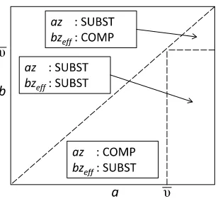
Next, consider how the shape of agent 1’s payoff function affects her incentives in choosing links and security. Increasing link intensity z˜ leads to greater benefits from tips through the AA term, but also to higher costs: both the explicit cost C³z,˜ f˜´and the “virus cost”BB (reflecting exposure to unblocked viruses) also rise. Notice that both the benefit and the virus cost terms are concave inz˜: each additional link yields a smaller marginal benefit from tips than the previous link, but also a smaller marginal harm from viruses. The logic is the same in both cases — the marginal effect of an additional link depends on the chance that the new link exposes an agent to a tip or virus, while all of her other links do not. An agent with many links is likely to already be exposed to the tip or virus, so the effect of the additional link is small. It might appear that in the absence of an explicit cost C³z,˜ f˜´, and with BB concave, the optimal choice of z˜ could run off toward infinity. In fact, one can show that that as long as some security is being provided (either by agent 1 or by the other agents), the marginal benefit from tips shrinks faster withz˜ than the marginal harm from viruses does, and this would limit link intensity even if there were no explicit costs associated with z˜. Notice also that AA−BB is convex in agent 1’s security level f˜. This makes sense after considering that an increase in f˜affects harm from viruses similarly to a reduction in ˜
z — both changes reduce her effective link intensity z˜ef f =
³
1−f˜´z˜. In both cases, removing an effective link at the margin has a smaller impact for a highly connected agent (z˜large orf˜small) because she is still likely to catch the virus via one of her other effective links. The convexity of the benefits from security tends to stack the deck against moderate levels of f˜; unless C³z,˜ f˜´ is also sufficiently convex, agents mayfind all or nothing security decisions (f˜= 1orf˜= 0) optimal. Finally, consider the interaction between aggregate properties of the network, like a and b, and individual incentives. First, unless other agents are sufficiently connected (z >1), aggregate connectivity will be nil (a = 0), and so there will be no benefit for agent 1 in forming links.
(az <˜ 2) a rise in total connectivity will tend to make marginal links more attractive for agent 1. Together, these two points constitute a positive network effect. However, if both the network and agent 1 individually are fairly saturated with connections (az >˜ 2), then a further rise inareduces the return to z˜. Thus we anticipate the positive network effect to be self-limiting.14 There is a similar relationship between unsecured connectivity and an individual agent’s effective links; we have ∂b∂∂z˜2
ef fBB = (2−bz˜ef f)Bbe
−bz˜ef f. Thus, when the network is relatively safe (bz˜
ef f <2), a
rise inbincreases the marginal harm to agent 1 from increasing linksz˜or reducing securityf˜. This tends to act against the positive network effect from tips, because when other agents add links, b
will rise, encouraging agent 1 to reduce z˜or increase f˜. However, in a relatively unsafe network (bz˜ef f >2), the incentivesflip — in this case, a shift by other agents toward more connected or less
secure behavior (and thus higherb) encourages agent 1 to become more connected and less cautious herself. Consequently, there may be a tendency for cautious or risky behavior in the network to be self-reinforcing.
4
Symmetric Equilibrium
In this section, we characterize the symmetric equilibria of a large decentralized economy under different cost structures. The sharpest results are obtained when security costs are extremely convex in f; we lead with the degenerate case in which security is free below a threshold f¯and infinitely costly above it. If we relax this to a smooth convex security cost, the results are similar, but it becomes harder to ensure that the necessary first order conditions for equilibrium are also sufficient. One complicating factor, as discussed earlier, is the convexity of benefits from security, which tempts agents toward all or nothing security decisions. Since this issue will be discussed in more depth when we consider elastic security costs, its treatment here will be brief.
Before turning to the case of step function security costs, consider the case in which C(z, f) is differentiable. If a symmetric equilibrium exists at the interior strategy(z, f), then agent 1’s payoff must satisfy the followingfirst order conditions:
∂ ∂z˜π1
³³
˜
z,f˜´; (z,f)−1´¯¯¯¯
(˜z,f˜)=(z,f)
= Aa2e−az−Bb2(1−f)e−(1−f)zb−Cz(z, f) = 0
∂ ∂f˜π1
³³
˜
z,f˜´; (z,f)−1´¯¯¯¯
(˜z,f˜)=(z,f)
= Bb2ze−(1−f)zb−Cf(z, f) = 0
and total and unsecured connectivity must be generated from individual choices according to a= 1−e−az and b= 1−e−(1−f)zb respectively. We can use these aggregation equations to write the first order conditions as
Aa2(1−a) = Cz(z, f) +
1−f
z Cf(z, f)
Bb2(1−b) = 1
zCf(z, f) 1 4Recall that1
−e−az˜can be interpreted as the probability that agent 1 connects to a non-negligible fraction of the population. Notice that the effect ofaon the marginal benefit fromz˜changes sign precisely when this probability is
This highlights two facts. First, at equilibrium, the cost of an increase in connections can be
represented by the direct cost Cz(z, f) plus the indirect cost of ‘sterilizing’ the increase in z with
an increase in f that is sufficient to hold (1−f)z constant. Second, the lefthand side of both equations makes it clear that an agent’s choices have the greatest impact on her connectivity when the network itself is moderately well connected (aand bnear 23).
4.1
Case 1: Inelastic Security Costs
As an idealization of a situation in which modest security measures are cheap, but additional measures are progressively more expensive, define C(z, f) as
C(z, f) =
(
0 iff ≤f¯
∞ iff >f¯
To avoid special cases, we will assume that f¯∈ (0,1). Under these costs, an agent will always choose as much free security as possible, so we replace the first order condition for security with the conditionf = ¯f.15 Since it is correct but confusing to refer to an increase inf¯as a decline in security costs, we will describe this equivalently as a rise in ‘security capacity.’ Given a strategy profile of ¡z,¯f¢
−1 for the other agents, agent 1’s marginal payofffrom z˜can be written as ∂
∂z˜π1
³¡
˜
z,f¯¢;¡z,¯f¢
−1 ´
=e−a˜z³Aa2−Bb2¡1−f¯¢e(a−(1−f¯)b)z˜´
It is clear that there always exists a trivial zero connection equilibrium: if z = 0, then a=b= 0, and z˜ = 0 is a weak best response for agent 1. We focus on the more interesting case in which
z > 1, so the network has strictly positive total connectivity. Note that because ¡1−f¯¢b < a,
the derivative is either negative for all z˜≥0 (if Aa2 ≤Bb2¡1−f¯¢) or switches from positive to negative exactly once. Thus, any strictly positive solution that we find to agent 1’s first order condition will be an optimal decision for her. This permits us to characterize equilibria as follows.
Proposition 3 Suppose a large decentralized economy has costs as described above, with security
capacity f¯. There exists a unique symmetric equilibrium with positive total connectivity. The
equilibrium strategy profile satisfiesz=−ln(1a−a) andf = ¯f, with aandbdetermined by the unique
(on (a, b)∈(0,1)2, b≤a) solution to the following pair of equations:
Aa2(1−a) = Bb2(1−b)¡1−f¯¢ (5)
1−f¯ = a
b
ln (1−b)
ln (1−a) (6)
Equation (5) represents the first order condition for links, interpreted in terms of the aggregate network variables a and b, and evaluated when link choices are symmetric. One can see again
1 5To be more precise, an agent strictly prefers higher security unlessb = 0, in which case she is indifferent. To
0 0.2 0.4 0.6 0.8 1 0
0.2 0.4 0.6 0.8 1
a b
A(a) = B (b)
0 0.2 0.4 0.6 0.8 1 0
0.25 0.5
Equilibria: B=2
a b
0.5 0.75 1
0 0.2 0.4 0.6 0.8 1
Equilibria: B = 0.9
a b
B = 1.1 B = 0.5 B = 0.9
f = 0.02
f = 0.5 f = 0.7
f = 0.5
f = 0.7 f = 0.2
f = 0.02
[image:22.612.99.549.71.216.2]f = 0.2 B = 5
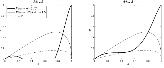
Figure 3: Equilibrium with security capacity f¯. Left: eqn. (7) at assorted values of B. (A = 1.) Middle and right: equilibrium condition (6) — dashed — at increasing values off¯, vs. (7).
that the marginal benefit from links interacts in a non-monotonic way with total connectivity a,
first rising, then falling. Likewise, the marginal harm from links is first rising and then falling in unsecured connectivity b. Equation (6) reflects the technological constraint specifying how total and unsecured connectivity must differ if agents choose security level f¯.
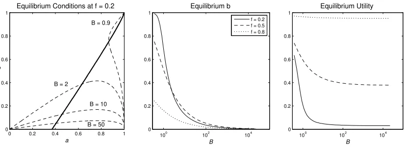
With inelastic security costs, the model has only two free parameters: the security capacity f¯, and the relative threat levelB/A. In order to illustrate their comparative static effects, it is useful to transform the equilibrium conditions so that the effects of f¯and B are separated. Substitute (6) into (5) to get
AΥ(a) =BΥ(b), (7)
where Υ(x) =−x(1−x) ln (1−x). Together, (7) and (6) are an equivalent representation of the equilibrium conditions, but now f¯and B/Aappear in separate equations. Examples of the curves defined by (7) and (6) are plotted in Figure 3.16 The function Υhas a natural interpretation. Set
Benef it(˜z) = Aa¡1−e−az˜¢ and Harm(˜z
ef f) =Bb
¡
1−e−bz˜ef f¢. We can recast the individual’s
decision problem as a maximization ofBenef it(˜z)−Harm(˜zef f) over total and effective
connec-tivity, z˜and z˜ef f, subject to the constraint thatz˜ef f/z˜= 1−f¯. Because an individual can make
a proportional increase or decrease in both types of connectivity without changing the value of the constraint, at an optimal decision the marginal benefit induced by a percentage increase inz˜must balance the marginal harm induced by a percentage increase inz˜ef f. That is
dBenef it(˜z)
dz/˜ z˜ =
dHarm(˜zef f)
dz˜ef f/z˜ef f
Evaluated at a symmetric profilez, we have
dBenef it(˜z)
dz/˜ z˜
¯ ¯ ¯ ¯ ˜
z=z
= Aza˜ 2e−a˜z¯¯z˜=z=
−ln(1a−a),e−az=1−a
=AΥ(a).
Similarly, BΥ(b) is the marginal harm, or −BΥ(b) the marginal payoff change, induced by a
1 6As the right panel of Figure 3 suggests, the most delicate part of the proof of Proposition 3 is to show existence