Munich Personal RePEc Archive
A quantile regression approach to bank
efficiency measurement
Mamatzakis, E and Koutsomanoli-Filippaki, Anastasia and
Pasiouras, Fotios
University of Sussex
12 March 2012
A quantile regression approach to bank efficiency
measurement
Anastasia Koutsomanoli-Filippaki
Bank of Greece, Greece
Emmanuel Mamatzakis
University of Sussex, UK
Fotios Pasiouras
University of Surrey, UK, and
Technical University of Crete, Greece
1. Introduction
The estimation of bank efficiency, whether at the branch or at the institution level, is a topic that
has attracted considerable attention in the literature (see Berger and Humphrey, 1997; Berger,
2007, Fethi and Pasiouras, 2010). Over the years a number of topics have been explored
including the relationship of efficiency with ownership (Miller and Parkhe, 2002), regulations
(Pasiouras, 2008), institutional development (Lensink et al., 2008), off-balance-sheet activities
(Siems and Clark, 1997), risk (Berger and DeYoung, 1997), stock returns (Chu and Lim, 1998),
mergers (Avkiran, 1999), and bank failure (Wheelock and Wilson, 2000) to name a few.
Despite the plethora of efficiency studies in the banking literature, there is no consensus
etc.) of fully efficient firms. For example, Berger and Humphrey (1997) mention that 69 of the
banking studies in their survey used nonparametric methods and 61 used parametric methods. In
general, data envelopment analysis (DEA) is the most widely used non-parametric technique,
and stochastic frontier analysis (SFA) is the most frequently employed parametric technique.
Each approach has its advantages and disadvantages and as a result it has supporters and equally
dedicated opponents. In general, the econometric approaches have the advantage of allowing for
noise in the measurement of the efficiency but their disadvantages are the imposition of a
particular production function form and the requirement of an assumption about the distribution
of efficiency. In contrast, the main advantages of DEA are that: (i) it avoids the need for a priori
specification of function forms, and (ii) it does not require any assumption to be made about the
distribution of inefficiency. One the other hand, the shortcomings of DEA are that: (i) it assumes
data to be free of measurement error, (ii) it is sensitive to outliers, (iii) having few observations
and many inputs and/or outputs will result in many firms appearing on the frontier.
Lately, a third approach was proposed in the literature, namely Quantile regression
analysis. This technique has been frequently employed in the econometrics literature; however,
there are only a few studies in the context of efficiency estimation examining among others the
efficiency of hotels (Bernini et al., 2004), nursing facilities (Knox et al., 2007), dairy farms
(Chidmi et al., 2011), and check processing operations (Wheelock and Wilson, 2008). In the case
of banking this techniques was applied only very recently, with a handful number of studies
examining US (Wheelock and Wilson, 2009), German (Behr, 2010) and European banks
(Koutsomanoli-Filippaki and Mamatzakis, 2011).
Quantile regression can be particular useful in the context of efficiency analysis. First,
in the firm level data (Behr, 2010). More detailed, the estimation of conditional quantiles is more
robust against outliers and it also provides the means to obtain different slope parameters
describing the production of efficient firms rather than average firms. Furthermore, as discussed
in Liu et al. (2008), quantile regression requires an assumption about the functional form of the
production frontier (unlike DEA); however, it does not require the imposition of a particular
form on the distribution of the inefficiency terms (unlike SFA). Additionally, quantile regression
avoids the criticism against DEA of not allowing for random error.
The present Chapter aims to provide an overview of this promising alternative approach, along
with an empirical application in a large international dataset, including 1,520 commercial banks
operating in 73 countries, between 2000 and 2006. Apparently, with such a wide coverage our
sample is quite heterogeneous both in terms of the countries’ development as well as in terms of
the banks’ characteristics. Given the increasing number of cross-country studies, our approach
provides an ideal setting for the application of quantile regression that can be particular useful in
samples with large bank heterogeneity. The next section discusses the methodological
framework of quantile regression. Then we present the empirical results. The concluding marks
are discussed in the last section.
2. Methodology
Quantile regression is a statistical technique intended to estimate, and perform inference about,
conditional quantile functions. This analysis is particularly useful when the conditional
distribution does not have a standard shape, such as an asymmetric, fat-tailed, or truncated
distribution. Consequently, quantile regression was recently employed in various strands of the
2012), the herding behavior in stock markets (Chiang et al., 2012), capital structure (Fattouh et
al., 2005), bankruptcy prediction (Li and Miu, 2010), ownership and profitability (Li et al.,
2009), the relationship between stock price index and exchange rate (Tsai, 2012), and credit risk
(Schechtman and Gaglianone, 2012).1 In the context of our study, quantile analysis provides an
ideal tool to examine bank efficiency heterogeneity, departing from conditional-mean models.
More detailed, the quantile regression approach allows efficient or almost efficient banks to
employ production relations that may differ strongly from the ones of average or low efficiency
banks, and in a sense it provides the means for the proper comparison with truly “benchmark”
banks that fall within the chosen quantile (Behr, 2010).
In detail, a quantile regression involves the estimation of conditional quantile functions,
i.e., models in which quantiles of the conditional distribution of the dependent variable are
expressed as functions of observed covariates (Koenker and Hallock, 2000). Using standard
formulation, the linear regression model takes the form:
φ
φ
ε
β
iit
it x
y = + (1)
where φ ∈(0, 1), xi is a K × 1 vector of regressors, xi βφ denotes the φth sample quantile of y
(conditional on vector xi), and εiφ is a random error whose conditional quantile distribution
equals zero.
The objective function for efficient estimation of β corresponding to the φth quantile of
the dependent variable (y) can be expressed by the following minimization problem:
⎭
⎬
⎫
⎩
⎨
⎧
−
−
+
−
∑
∑
≤≥ β β
β
φ
β
φ
β
i i i
i i y x
i i x y i i
i
x
y
x
y
n
: :)
1
(
1
min
(2)which is solved via linear programming. Note that the median estimator, that is, quantile
regression estimator for φ = 0.5, is similar to the least-squares estimator for Gaussian linear
models, except that it minimizes the sum of absolute residuals rather than the sum of squared
residuals.
For the estimation of efficiency we opt for a parametric methodology and employ the
Distribution-free approach (DFA), developed by Berger (1993), who follows Schmidt and
Sickless (1984). This approach is a particularly attractive technique due to its flexibility as it
does not impose a-priori any specific shape on the distribution of efficiency (DeYoung, 1997).
Instead, the DFA methodology assumes that the inefficiency of each bank remains constant
across the sample period and that random error averages out over time.
By averaging the residuals to estimate bank-specific efficiency, DFA estimates how well
a bank tends to do relative to its competitors over a range of conditions over time, rather than its
relative efficiency at any one point in time (DeYoung, 1997). Berger and Humphrey (1997)
argue that the DFA approach gives a better indication of a bank’s longer-term performance by
averaging over a number of conditions, than any of the other methods. Therefore, under DFA a
panel data is required and only panel estimates of efficiency over the entire time interval are
available.2
For the estimation of the Distribution-free approach we opt for the widely used translog
cost function, which gives us the following specification:
lnCi = α0 +
∑
i
i
i P
a ln +
∑
i
i
Y ln
i
β
+ ½∑∑
i j
i
ij P Pj
a ln ln +½
∑∑
Υ Υ i jj ijln i ln
β +
∑∑
Υi j
j i
ijlnPln
δ +
∑
i
i
ilnΝ
φ +½
∑∑
i
ijln ln
j
j i N N
φ +
∑∑
i j j i N Pln ln ij ξ
∑∑
+ i j j i N Y ln ln ijζ + kDi+ lnvi +ln ui (3)
where all variables are expressed in natural logs.3 Cit denotes observed total cost for bank i, Pi is
a vector of input prices Yj is a vector of bank outputs, and N is a vector of fixed netputs4.
Moreover, because structural conditions in banking and general macroeconomic conditions may
generate differences in banking efficiency from country to country, we also include country
effects in the estimation of the cost frontier. Note that ui is the bank specific efficiency factor and
vi is the random error term. All elements of Equation (3) are allowed to vary across time with the
exception of ui, which remains constant for each bank by assumption. In the estimation, the lnvi
and ln ui terms are treated as a composite error term, i.e., lnεˆi =lnvˆi +lnuˆi. Once estimated the
residuals, ln
ε
ˆi, are averaged across T years for each bank i. The averaged residuals areestimates of the X-efficiency terms, ln ui , because the random error terms, lnvi, tend to cancel
each other out in the averaging. Thus, bank’s i efficiency is defined as:
(DeYoung, 1997). Following the empirical literature, the 7-year period of our sample reasonably balances these concerns.
3 Standard homogeneity and symmetry restrictions are imposed:
∑
= ii
a 1,
∑
= iij
a 0,
∑
=i
ij 0
δ ,
∑
=i
ij 0
ξ , αim =
αmiand αjk= αkj, ∀i,j,k,m.
)] ˆ ln ˆ exp[(ln ) ˆ exp[(ln ) ( ˆ exp[([ )] ˆ exp[(ln ) ( ˆ exp[ min min i i i i i i
i u u
u y p f u y p f
EFF = = − (4)
where lnuˆiis the residual vector after having averaged over time and lnuˆmin is the most
efficient bank in the sample.
2.3. Data and specification of the frontier
We start the construction of our dataset by considering all the commercial banks in the
Bankscope database. Once we exclude banks for which we do not have complete data for the
period of our study, we end up with a sample of 1,520 commercial banks operating in 73
countries, between 2000 and 2006. This sample includes domestic and foreign banks as well as
listed and unlisted banks. It is worth emphasizing that there exists certain degree of heterogeneity
across banks as they operate in quite different environments in terms of regulations, institutional
infrastructure, market characteristics, and overall development. Despite the bank heterogeneity ,
it is not uncommon for the recent bank efficiency literature to use such large international
datasets (e.g. Lensink et al., 2008; Barth et al., 2010), making our setting ideal for testing the
usefulness of a quantile approach. As discussed in the next section, to reveal potential
differences across different levels of development, we combine information from the
International Monetary Fund (IMF) and the European Bank for Reconstruction and Development
(EBRD), and we classify banks in four groups according to the level of development of the
country that they operate, namely major advanced countries, advanced countries, transition
countries, and developing countries. Moreover to examine the impact of the aforementioned
country-specific characteristics we use information from various sources such as the Worldwide
and the World Bank database on Financial Development and Structure and we perform
second-stage regressions. These are results are discussed in detail in section 3.2.
There is a debate in the literature as for the selection of inputs and outputs, and in
particular as for the appropriate treatment of deposits (Berger and Humphrey, 1997). Following
Dietsch and Lozano-Vivas (2000), Maudos et al. (2002), Pasiouras et al. (2009), and others, we
adopt the value added approach which suggests using deposits as outputs since they imply the
creation of value added. Therefore, we use the following three outputs: loans (Y1), other earning
assets (Y2), and total deposits (Y3). Furthermore, consistent with numerous studies on bank
efficiency we select the following three input prices: cost of borrowed funds (P1), calculated as
the ratio of interest expenses to total deposits; cost of labour (P2), calculated by dividing the
personnel expenses by total assets; and cost of physical capital (P3), calculated by dividing the
expenditures on plant and equipment (i.e. overhead expenses net of personnel expenses) by fixed
assets. Thus, our approach recognizes that deposits have both input and output characteristics,
the first captured through the inclusion of the interest expense paid on deposits in the input prices
vector, the second captured through the stock of deposits in the output vector.
Furthermore, we normalize the dependent variable and the three outputs by equity.
Berger et al. (2000) point out that the normalization by equity capital controls for
heteroskedasticity, reduces scale biases in estimation, it provides the grounds for a more
economic interpretation, and it controls for financial leverage.
Additionally, to account for technological differences across different levels of a
country’s overall development, we use dummy variables to distinguish between major advanced,
3. Empirical results
3.1 Cost efficiency estimates
We calculate cost efficiency scores for each bank in our sample using the
Distribution-free approach and compare these scores across quantiles and across different levels of
development. In order to cover as wide range of quantiles as possible, we run regressions for
[image:10.612.128.484.357.580.2]quantiles 0.05, 0.25, 0.75 and 0.95.
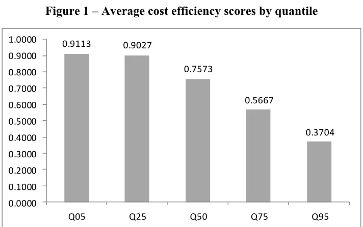
Figure 1 – Average cost efficiency scores by quantile
0.9113 0.9027
0.7573
0.5667
0.3704
0.0000 0.1000 0.2000 0.3000 0.4000 0.5000 0.6000 0.7000 0.8000 0.9000 1.0000
Q05 Q25 Q50 Q75 Q95
Source: Authors’ estimations.
Figure 1 presents the average efficiency scores across quantiles. There are three
interesting observations to be made. First, there is a remarkable variation across quantiles. More
to 0.9113 for quantile 0.05. Second, cost efficiency estimates across quantiles, and particularly in
the tail of the distribution, differ substantially from the conditional mean (OLS) point estimate of
efficiency, which is approximated by quantile 0.5 and equals 0.7573. Thus, quantile regression
analysis provides a more comprehensive picture of the underlying range of disparities in cost
efficiency than the classical estimation. Third, the average efficiency is monotonically
decreasing as it follows a negative trend at higher order of quantiles. More detailed, cost
efficiency is estimated at around 0.9113 for quantile 0.05, decreases to 0.9027 for quantile 0.25,
dropping further to 0.7573 and 0.5667 for quantiles 0.50 and 0.75 respectively, while it reaches
its minimum value at 0.3704 when the cost function is calculated at the 0.95 quantile. In general,
these results confirm the ones of Koutsomanoli-Filippaki and Mamatzakis (2011) for European
banks; however, the minimum cost efficiency in our case is considerably lower than the one
[image:11.612.103.507.470.686.2]recorded in their study.
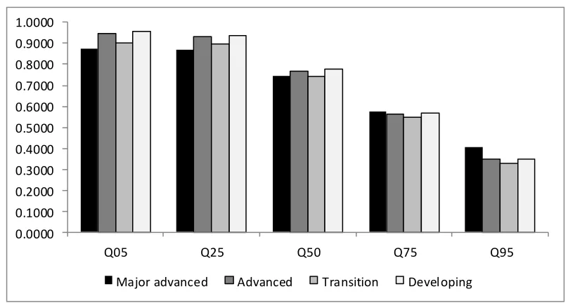
Figure 2 – Average cost efficiency scores by country development level and quantiles
0.0000 0.1000 0.2000 0.3000 0.4000 0.5000 0.6000 0.7000 0.8000 0.9000 1.0000
Q05 Q25 Q50 Q75 Q95
Major advanced Advanced Transition Developing
Figure 2 presents a disaggregation of the estimated cost efficiencies by the level of a
country’s overall development (i.e. major advanced, advanced, etc.). First, this disaggregation
confirms the aforementioned negative trend at higher order of quantiles, irrespective of the level
of overall country development. Second, there appears to some variability in the underlying
relationship between the level of a country’s overall development and the cost efficiency of
banks. More detailed, we observe that banks operating in major advanced countries appear to be
less cost efficient when looking at the 0.05 and 0.25 quantiles, and more cost efficient when
looking at the 0.75 and 0.95 quantiles. Additionally, the scores appear of similar magnitude when
looking at the 0.50 quantile. This would imply that resolving into the classical OLS mean
regression analysis would result to loss of valuable information regarding the bank performance
across the world. Finally, the average cost efficiency of banks from major advanced countries is
always higher than that of banks from all other categories the highest quantile, but the former
becomes lower than that the latter at very low quantiles , i.e. Q5 and Q25. The differences in
cost efficiency between advanced, transition and developing countries remain quite stable across
quantiles, whilst they are not large in magnitude. It is worth noticing that countries in transition
have a record of the lowest bank performance in our sample. This evidence suggests that reform
efforts during transition could come at the expense of lowering bank cost efficiency, though once
the country becomes advanced the benefits of these reforms translate into higher scores in cost
efficiency.
Table 1 presents the spearman’s rank correlation coefficients between the cost efficiency
depending on whether we compare the rankings that are obtained from estimations at
[image:13.612.112.503.160.586.2]neighboring or distant quantiles.
Table 1 – Spearman’s rank correlation coefficients
All sample Q05 Q25 Q50 Q75 Q95
Q05 1.000
Q25 0.908*** 1.000
Q50 0.692*** 0.794*** 1.000
Q75 0.230*** 0.356*** 0.644*** 1.000
Q95 -0.217*** -0.088*** 0.203*** 0.580*** 1.000
Major advanced countries Q05 Q25 Q50 Q75 Q95
Q05 1.000
Q25 0.920*** 1.000
Q50 0.661*** 0.794*** 1.000
Q75 -0.013 0.147*** 0.477*** 1.000
Q95 -0.567*** -0.417*** -0.045 0.574*** 1.000
Advanced countries Q05 Q25 Q50 Q75 Q95
Q05 1.000
Q25 0.414*** 1.000
Q50 0.659*** 0.348*** 1.000
Q75 0.581*** 0.266*** 0.800*** 1.000
Q95 0.464*** 0.634*** 0.620*** 0.545*** 1.000
Transition countries Q05 Q25 Q50 Q75 Q95
Q05 1.000
Q25 0.709*** 1.000
Q50 0.439*** 0.744*** 1.000
Q75 0.172** 0.665*** 0.699*** 1.000
Q95 -0.118* 0.514*** 0.620*** 0.907*** 1.000
Developing countries Q05 Q25 Q50 Q75 Q95
Q05 1.000
Q25 0.948*** 1.000
Q50 0.862*** 0.911*** 1.000
Q75 0.717*** 0.791*** 0.915*** 1.000
Q95 0.587*** 0.697*** 0.773*** 0.848*** 1.000
Notes: ***Statistically significant at the 1% level, **Statistically significant at the 5% level, *Statistically significant at the 10% level
For example, estimations at the 0.05 and 0.25 quantiles rank the banks in approximately
the same way. Additionally, there are moderate correlations between estimations at the 0.50
However, there are remarkable differences between estimations at the 0.05 and 0.95 quantile, as
well as between the 0.25 and 0.95 quantiles, as it becomes evident by the negative coefficients.
The correlations by level of development reveal the existence of differences across the group of
countries. For example, the estimations for major advanced and transition countries are similar to
the ones for the whole sample. Nonetheless, in the case of developing countries we observe that
not only the correlation coefficients tend to be higher but there is also a moderate positive
correlation between estimations at 0.05 and 0.95 quantiles. In the case of advanced countries, the
correlations are similar to the ones of developing countries, although lower in magnitude.
3.2 Determinants of cost efficiency
To shed more light into our analysis we also perform second-stage regressions, where
cost efficiency scores derived at different quantiles are regressed on a set of environmental
variables. Following recent studies by, among others, Pasiouras (2008), Pasiouras et al. (2009),
Lozano-Vivas and Pasiouras (2010) we account for regulatory conditions using four indices that
control for capital requirements (CAPRQ), private monitoring (PRMONIT), supervisory power
(SPOWER), and activity restrictions (ACTRS). To capture the macroeconomic conditions we
use the inflation rate (INFL) and real GDP growth (GDPGR). To account for industry conditions
we use the ratio of bank claims to the private sector over GDP (CLAIMS), and concentration in
the banking sector (CONC). Finally, to control for the institutional development (INSTDEV) we
use the average of six indicators measuring voice and accountability, political stability,
government effectiveness, regulatory quality, rule of law, and control of corruption (see e.g.
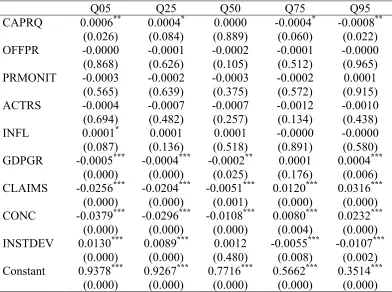
The results in Table 2 reveal various interesting findings. First, the 0.75 and 0.95
quantiles appear to be of significance for the direction of the impact of various environmental
variables on cost efficiency. Moreover, the positive impact of CAPRQ on cost efficiency that is
reported at the 0.05 and 0.25 quantiles is reversed at the 0.75 and 0.95 quantiles. This change in
the sign of CAPRQ has important implications as it shows that capital requirements have a
positive influence on the more efficient banks and a negative impact on the less efficient banks.
Thus, either the most efficient banks are capable of turning the regulatory burden imposed by
higher capital requirements to their benefit or supervisors distinguish between efficient and
inefficient banks. The latter would be in line with the results of DeYoung et al. (2001) who
conclude in their US study that “…regulators impose greater discipline and higher distress costs
on inefficient banks than on efficient banks” (p. 275). The impact of the institutional
development also differs across quantiles, being positive for the more efficient banks and
negative for the less efficient banks.
In contrast, GDPGR, CLAIMS and CONC exercise a negative influence on the efficiency
of banks in the case of the 0.05 and 0.50 quantiles and a positive impact in the case of the 0.75
and 0.95 quantiles. The negative impact of GDP growth is in line with the findings of Maudos
(2002) who argue that under expansive demand conditions, banks feel less pressured to control
their costs and are therefore, less cost efficient. However, our results illustrate that there is a
turning point after which banks are cautious and they take advantage of the growth in the
economy so that they will operate more efficiently. The similar picture that emerges in the case
on efficiency, are mixed.5 Overall our findings indicate that an OLS analysis, which is close to
the median quantile (0.5), would be misleading, as it would report an insignificant coefficient for
capital requirements (CAPRQ) and institutional development (INSTDEV), and it would also
[image:16.612.111.503.247.539.2]ignore that the impact of environmental factors can vary across different levels of efficiency.
Table 2 – 2nd stage regressions
Q05 Q25 Q50 Q75 Q95
CAPRQ 0.0006**
(0.026) 0.0004* (0.084) 0.0000 (0.889) -0.0004* (0.060) -0.0008** (0.022)
OFFPR -0.0000
(0.868) -0.0001 (0.626) -0.0002 (0.105) -0.0001 (0.512) -0.0000 (0.965)
PRMONIT -0.0003
(0.565) -0.0002 (0.639) -0.0003 (0.375) -0.0002 (0.572) 0.0001 (0.915)
ACTRS -0.0004
(0.694) -0.0007 (0.482) -0.0007 (0.257) -0.0012 (0.134) -0.0010 (0.438)
INFL 0.0001*
(0.087) 0.0001 (0.136) 0.0001 (0.518) -0.0000 (0.891) -0.0000 (0.580)
GDPGR -0.0005***
(0.000) -0.0004*** (0.000) -0.0002** (0.025) 0.0001 (0.176) 0.0004*** (0.006)
CLAIMS -0.0256***
(0.000) -0.0204*** (0.000) -0.0051*** (0.001) 0.0120*** (0.000) 0.0316*** (0.000)
CONC -0.0379***
(0.000) -0.0296*** (0.000) -0.0108*** (0.000) 0.0080*** (0.004) 0.0232*** (0.000)
INSTDEV 0.0130***
(0.000) 0.0089*** (0.000) 0.0012 (0.480) -0.0055*** (0.008) -0.0107*** (0.002) Constant 0.9378***
(0.000) 0.9267*** (0.000) 0.7716*** (0.000) 0.5662*** (0.000) 0.3514*** (0.000)
Notes: ***Statistically significant at the 1% level, **Statistically significant at the 5% level, *Statistically significant at the 10% level; p-values in parentheses; Results obtained from fixed effects estimations with the dependent variable being the cost efficiency at different quantiles; Variables are defined in Appendix I
5
4. Conclusions
This Chapter presents an application of quantile regression analysis in estimating the cost
efficiency of 1,520 commercial banks operating in 73 countries during 2000-2006. This approach
allows us to estimate banks’ cost function for various quantiles of the conditional distribution
and to examine the tail behaviours of that distribution. In further analysis we also examine
whether and how the impact of environmental factors differs across the various quantiles of
efficiency. The employed methodological framework is of particular importance in light of the
heterogeneity in bank efficiency across various countries.
The results can be summarized as follows. First, there is a remarkable variation of
efficiency across quantiles. Second, the efficiency estimates across quantiles, and particularly in
the tail of the distribution, differ substantially from the conditional mean (OLS) point estimate of
efficiency (i.e. quantile 0.5). Third, the average efficiency is monotonically decreasing. We
confirm this negative trend at higher order of quantiles for all levels of overall country
development (i.e. major advanced, advanced, transition, developing countries). Fourth, there
appears to be some variability regarding the underlying relationship between the level of a
country’s overall development and bank cost efficiency. Fifth, the results of spearman’s rank
correlation coefficients show that there exist variability in the ranking of banks depending on
whether we compare estimations from neighboring or distant quantiles. In this case, the results
differ among different levels of overall country development. Sixth, the estimations of the
second stage regressions illustrate that there is turning point as for the direction of the impact of
various variables on cost efficiency. Furthermore, our findings indicate that an OLS analysis,
quantile regressions by permitting the estimation of various quantile functions of the underlying
conditional distribution provide a more comprehensive picture of the underlying relationships.
References
Avkiran, N.K. (1999) The evidence on efficiency gains: The role of mergers and the benefits to
the public. Journal of Banking and Finance, 23, 991-1013.
Barth, J.R., Lin, C., Ma, Y., Seade, J., and Song, F.M. (2010) Do Bank Regulation, Supervision
and Monitoring Enhance or Impede Bank Efficiency?, Available at SSRN:
http://dx.doi.org/10.2139/ssrn.1579352
Behr, A. (2010) Quantile regression for robust bank efficiency score estimation. European
Journal of Operational Research, 200, 568-581.
Berger, A. (1993) Distribution-free estimates of efficiency in the US banking industry and tests
of the standard distribution assumptions. Journal of Productivity Analysis,4, 261-292.
Berger, A. and Humphrey, D. (1997) Efficiency of financial institutions: international survey and
direction of future research. European Journal of Operational Research, 98, 175-212.
Berger, A.N. (2007) International Comparisons of Banking Efficiency. Financial Markets,
Institutions & Instruments, 16, 119- 144.
Berger, A.N. and DeYoung, R. (1997) Problem loans and cost efficiency in commercial banks.
Journal of Banking and Finance, 21, 849-870.
Berger, A.N. and Mester, L.J. (1997) Inside the black box: what explains differences in the
efficiencies of financial institutions? Journal of Banking and Finance,21, 895-947.
Berger, A.N., Cummins, J.D., Weiss, M.A., and Zi, H. (2000) Conglomeration versus Strategic
Focus: Evidence from the Insurance Industry. Journal of Financial Intermediation, 9, 323-362.
Bernini, C., Freo, M. and Gardini, A. (2004) Quantile estimation of frontier production function.
Chiang, T.C., Li, J., and Tan, L. (2010) Empirical investigation of herding behavior in Chinese
stock markets: Evidence from quantile regression analysis. Global Finance Journal, 21, 111-124.
Chidmi, B., Solís, D. and Cabrera, V.E. (2011) Analyzing the sources of technical efficiency
among heterogeneous dairy farms: A quantile regression approach. Journal of Development
and Agricultural Economics,3, 318-324.
Chu, S.F. and Lim, G.H. (1998) Share performance and profit efficiency of banks in an
oligopolistic market: evidence from Singapore. Journal of Multinational Financial
Management, 8, 155–168.
DeYoung, R. (1997) A diagnostic test for the distribution-free efficiency estimator: An example
using U.S. commercial bank data, European Journal of Operational Research, 98, 243-249.
Dietsch, M. and Lozano-Vivas, A. (2000). How the environment determines banking efficiency:
a comparison between French and Spanish industries. Journal of Banking and Finance, 24, 985-1004.
Fattouh, B., Scaramozzino, P. and Harris, L. (2005) Capital structure in South Korea: a quantile
regression approach. Journal of Development Economics, 76, 231-250.
Fethi, M.D. and Pasiouras, F. (2010) Assessing bank efficiency and performance with
operational research and artificial intelligence techniques: A survey. European Journal of
Operational Research, 204, 189-198.
Fries, S. and Taci, A. (2005) Cost efficiency of banks in transition: Evidence from 289 banks in
15 post-communist countries. Journal of Banking and Finance, 29, 55-81.
Grigorian, D.A. and Manole, V. (2006) Determinants of Commercial Bank Performance in
Transition: An Application of Data Envelopment Analysis. Comparative Economic Studies,
48, 497-522.
Klomp, J. and de Haan, J. (2012) Banking risk and regulations: Does one size fit all? Journal of
Knox, K.J., Blankmeyer, E.C. and Stutzman, J. R. (2007) Technical efficiency in Texas nursing
facilities: A stochastic production frontier approach. Journal of Economics and Finance, 9, 75-86.
Koenker, R. and Hallock, K. (2000) Quantile Regression: An Introduction. Available at
http://www.econ.uiuc.edu/~roger/research/intro/intro.html.
Koenker, R. and Hallock, K.F. (2001) Quantile Regression, Journal of Economic Perspectives,
15, 143-156.
Koutsomanoli-Filippaki, A.I. and Mamatzakis, E.C. (2011) Efficiency under quantile regression:
What is the relationship with risk in the EU banking industry? Review of Financial
Economics, 20, 84-95.
Lensink, R., Meesters, A. and Naaborg, I. (2008) Bank efficiency and foreign ownership: do good
institutions matters? Journal of Banking and Finance, 32, 834-844.
Li, M-Y. L. and Miu, P. (2010) A hybrid bankruptcy prediction model with dynamic loadings on
accounting-ratio-based and market-based information: A binary quantile regression
approach. Journal of Empirical Finance, 17, 818-833
Li, T., Sun, L. and Zou, L. (2009) State ownership and corporate performance: A quantile
regression analysis of Chines listed companies. China Economic Review, 20, 703-716.
Lozano-Vivas, A. and Pasiouras, F. (2010). The impact of non-traditional activities on the
estimation of bank efficiency: International evidence. Journal of Banking and Finance, 34, 1436-1449.
Maudos, J., Pastor, J.M., Perez, F. and Quesada, J. (2002) Cost and profit efficiency in European
banks. Journal of International Financial Markets, Institutions and Money, 12, 33-58.
Mester, L.J. (2003) Applying efficiency measurement techniques to central banks. Working
Paper 3-25, Pennsylvania: Wharton Financial Institutions Centre.
Miller, S.R. and Parkhe, A. (2002) Is there a liability of foreignness in global banking? An
empirical test of banks’ X-efficiency. Strategic Management Journal, 23, 55-75.
Pasiouras, F. (2008) International evidence on the impact of regulations and supervision on banks’
technical efficiency: an application of two-stage data envelopment analysis. Review of
Pasiouras, F., Tanna, S. and Zopounidis, C. (2009) The impact of banking regulations on banks'
cost and profit efficiency: Cross-country evidence. International Review of Financial
Analysis, 18, 294-302.
Schechtman, R. and Gaglianone, W.P. (2012) Macro stress testing of credit risk focused on the
tails. Journal of Financial Stability, 8, 174-192.
Schmidt, P. and Sickles, R. (1984) Production frontiers and panel data. Journal of Business and
Economic Statistics,2, 367-374.
Siems, T.F. and Clark, J.A. (1997) Rethinking Bank Efficiency and Regulation: How
Off-Balance-Sheet Activities Make a Difference. Federal Reserve Bank of Dallas Financial
Industry Studies, December, 1-12.
Tsai, I-C. (2012)The relationship between stock price index and exchange rate in Asian markets:
A quantile regression approach. Journal of International Financial Markets, Institutions
and Money, 22, 609-621
Wheelock, D.C. and Wilson, P.W. (2000) Why do banks disappear? The determinants of U.S.
bank failures and acquisitions. Review of Economics and Statistics, 82, 127–138.
Wheelock, D.C. and Wilson, P.W. (2008) Non-parametric, unconditional quantile estimation for
efficiency analysis with an application to Federal Reserve check processing operations.
Journal of Econometrics, 145, 209–225.
Wheelock, D.C. and Wilson, P.W. (2009) Robust Nonparametric Quantile Estimation of
Efficiency and Productivity Change in U.S. Commercial Banking, 1985–2004. Journal of