On a Non Definite Sturm Liouville Problem in the Two Turning Point Case—Analysis and Numerical Results

http://www.scirp.org/journal/jamp ISSN Online: 2327-4379

ISSN Print: 2327-4352

On a Non-Definite Sturm-Liouville Problem in the

Two-Turning Point Case—Analysis and Numerical

Results

Mervis Kikonko1,2

1_{Department of Engineering Sciences and Mathematics, Luleå University of Technology, Luleå, Sweden} 2_{Department of Mathematics and Statistics, The University of Zambia, Lusaka, Zambia}

Abstract

In this paper, we study the non-definite Sturm-Liouville problem comprising of a regular Sturm-Liouville equation and Dirichlet boundary conditions on a closed in-terval. We consider the case in which the weight function changes sign twice in the given interval of definition. We give detailed numerical results on the spectrum of the problem, from which we verify various results on general non definite Sturm- Liouville problems. We also present some theoretical results which support the nu-merical results. Some nunu-merical results seem to be in contrast with the results that are so far obtained in the case where the weight function changes sign once. This leads to more open questions for future studies in this particular area.

Keywords

Eigenvalue, Eigenfunction, Non-Definite, Turning Point, Richardson Number, Richardson Index, Haupt Index, Oscillation Number, Right-Definite, Left-Definite

1. Introduction

The regular Sturm-Liouville problem involves finding the values of a parameter λ (generally complex) for which the equation

( ) ( )

(

p x u x′

)

' q x u x

( ) ( )

λw x u x

( ) ( )

− + = (1)

has a solution u (non-identically zero) in

( )

a b, satisfying the boundary conditions

(2)-(3) below.

( )

cos

( )( )

sin 0,

u a α− pu′ a α = (2) How to cite this paper: Kikonko, M. (2016)

On a Non-Definite Sturm-Liouville Problem in the Two-Turning Point Case—Analysis and Numerical Results. Journal of Applied Mathematics and Physics, 4, 1787- 1810. http://dx.doi.org/10.4236/jamp.2016.49184

Received: July 22, 2016 Accepted: September 25, 2016 Published: September 28, 2016

Copyright © 2016 by author and Scientific Research Publishing Inc. This work is licensed under the Creative Commons Attribution International License (CC BY 4.0).

( )

cos

( )( )

sin 0,

u b β+ pu′ b β= (3)

, , 0 , π.

a≤ ≤ − ∞ < < < +∞ ≤x b a b α β < The parameter λ is called an eigenvalue

and the corresponding function u is called an eigenfunction. The set consisting of all the eigenvalues of the problem consisting of (1) and the boundary conditions (2)-(3) is called the spectrum. The coefficient functions are such that p q w, , :

[ ]

a b, →, py′

is absolutely continuous in

( )

a b, , and 1 1

( )

, ,q w L a b, .

p ∈ In what follows (,) denotes

the inner product of the Hilbert space 2

[ ]

,

L a b . A point at which the weight function

( )

w x changes sign is called a turning point. The number of zeros that an eigen-

function has within the open interval

( )

a b, , is called the oscillation number of the

corresponding eigenvalue. In this paper, the setting is that u_n

( )

x =u x

(

,λ_n

)

has

exactly n zeros in

( )

a b, . That is, λn has oscillation number n.

Definition 1. Suppose that the eigenfunctions of a Sturm-Liouville problem are ordered according to increasing eigenvalues of the problem, the eigenfunctions are said to have the interlacing property, if between two zeros of the eigenfunction un lies

exactly one zero of the eigenfunction un+1.

Definition 2. A homogeneous linear differential equation

( )

_{( )}

( )1

_{( )}

1 0

n n

n

Ly=y +p x y − ++p x y=

of order n is called disconjugate on an interval I if no non-trivial solution has n zeros on I, multiple zeros being counted according to their multiplicity.

We pronounce that the strong interest of this field during all these years is that this theory is important in Applied Mathematics, where SL problems occur very commonly. The differential equations considered here arise directly as mathematical models of motion according to Newton’s law, but more often as a result of using the method of separation of variables to solve the classical partial differential equations of physics, such as Laplace’s equation, the heat equation, and the wave equation, (see e.g [1]). Let (1) be written as

( )

( )

d d

, where .

d d

Tu wu T p x q x x x

λ  

= = − _{ }+

  (4)

Then, the problem consisting of (4) and the boundary conditions (2)-(3) is called right-definite if the form

(

)

2

, d

b

a

wu u =

∫

w u x (5)

is definite. In this case there is a sequence

{ }

λn of real eigenvalues such that

0 1 n

λ λ λ

−∞ < < <_< <_

and λ → ∞n as n→ ∞, with a finite number of negative eigenvalues (see e.g, [2][3]).

If the form

(

)

( )

2

( )

2

(

( )

2

( )

2

)

, cot cot d

b

a

is definite for each u≠0, the problem is called left-definite. In this case the problem consists of two sequences of eigenvalues

{ }

λn

± _{such that}

n

λ±_{→ ±∞ as} .

n→ ∞ If we

let λ0 to be a real eigenvalue with smallest absolute value, then in the left- and right-

definite case, the corresponding eigenfunction has no zero in

( )

a b, . When neither

(

Tu u,

)

nor

(

wu u,

)

is definite, then the problem is called non-definite (indefinite).

In this paper our focus is on a non-definite Sturm-Liouville problem in which the weight function w x

( )

has two turning points in the interval of definition.

The Non-Definite (or Indefinite) Case

Here we give a summary on the non-definite case, detailed literature can be found in the papers [3]-[9], etc, and the references there in. In the non-definite case the spectrum is discrete, always consists of a doubly infinite sequence of real eigenvalues, and has at most a finite and even number of non-real eigenvalues (necessarily occurring in complex conjugate pairs).

Remark 1. If the problem consisting of the equation

( ) ( )

(

p x u x′

)

' q x u x

( ) ( )

λu x

( )

, λ 0

− + = ≠ ₍₇₎

and the boundary conditions (2)-(3) has N distinct negative eigenvalues, then the number of distinct pairs of non-real eigenvalues of the problem (1)-(3) cannot exceed N.

For more details on remark 1, we refer the interested reader to the papers [2]

(Theorem 4.2.1), [3] (Theorem 2), [10] (Corollary 1.7), and the references there. In the non-definite case, as Richardson [4] puts it, the march of the zeros is not monotone with λ∈_{ (in contrast with the left- and right-definite cases). In fact there may be a} range of values of λ such that as λ increases, the number of zeros first decreases, then increases, then decreases and finally increases, the minimum number being a positive integer. As a result the eigenfunction corresponding to the eigenvalue λ0 can

have any number of zeros in

( )

a b, in contrast with the definite case, that is to say, a

non-definite Sturm-Liouville problem will tend not to have a real ground state (positive eigenfunction). In relation to this behaviour of the real spectrum of the non-definite Sturm-Liouville problem, Mingarelli [6] defines two types of indexes which are due to Richardson [4] and Haupt [11].

Theorem 1. ([6] Haupt-Richardson Oscillation Theorem)

In the non-definite case of (1)-(3), there exists an integer nR≥0 such that for each

R

n≥n there are at least two real solutions of (1)-(3) having exactly n zeros in

( )

a b,

while for n<nR there are no real solutions having n zeros in

( )

a b, . Furthermore

there exists a possibly different integer nH ≥nR such that for each n≥nH there are

precisely two solutions having exactly n zeros in

( )

a b, .

Mingarelli [6] calls nR and nH the Richardson Index and Haupt Index, respec-

tively. If we consider positive eigenvalues separately, we can define for all λ>0, an integer n_R+≥0, such that for each n≥n_R+, there is at least one real solution of the

having n zeros. Also, there is an integer nH 0

+ _{≥ such that for each}

H

n≥n+ , there is

exactly one real solution having precisely n zeros in

( )

a b, , while for n<n_H+, there

are no solutions having n zeros in

( )

a b, . Analogue for λ<0 defines nR

− _and

H n− .

Furthermore, for real λ _{there exist two numbers} λ+ _{and λ}− _{called the Richardson}

numbers defined as

(

) ( )

{

2

}

inf : , b , d 0 , 0

a u x w x x

λ+ ₌ ρ_{∈ ∀ >}λ ρ λ _{> ∀ >}λ

∫



(

) ( )

{

2

}

sup : , b , d 0 , 0.

a u x w x x

λ−₌ ρ_{∈ ∀ <}λ λ _{< ∀ <}λ

∫

 

We note that

H

n

λ+ <λ+ . We can interpret λ+ as the smallest number such that the real eigenvalues greater than λ+ _{behave as in a “typical” Sturm-Liouville problem,}

that is, an eigenvalue is uniquely associated with its oscillation number, and λ− _is

interpreted similarly [7]. We note that in the right-definite case, λ+=λ−= −∞, while

in the left-definite case, λ+=λ−=0. As Jabon and Atkinson [7] rightly put it, in the non-definite case, the determination of these numbers is a very significant problem.

Theorem 2. ([3] Theorem 3)

Let λ _and u x

₍

,λ

₎

be a non-real eigenvalue and associated non-real eigenfunction

of problems (1)-(3). If w x

( )

has precisely n turning points in

( )

a b, then u x

(

,λ

)

may vanish at most

(

n−1

)

-times in

( )

a b, .

Corollary 1. (Corollary 1 [3])

Let λ _and u x

₍

,λ

₎

be a non-real eigenvalue and associated non-real eigenfunction

of problems (1)-(3). If w x

( )

has exactly one turning point in

( )

a b, then u x

(

,λ

)

≠0

in

( )

a b, .

In relation to corollary 1, we state the following theorem which is due to Richardson

[4], see also the papers [3][6].

Theorem 3. (Richardson’s Oscillation theorem)

Let w be continuous and not vanish identically in any right neighborhood of x=a. If w x

( )

changes its sign precisely once in

( )

a b, then the roots of the real and

imaginary parts φ _and ϕ _{of any non-real eigenfunction} u= +φ ϕi corresponding

to a non-real eigenvalue, separate one another (or interlace).

Below are some of the many open questions that Mingarelli in [3] [6] raises on non-definite or indefinite Sturm-Liouville problems.

1) Estimate the oscillation numbers nR

+ _and

H

n+ in terms of the given data , , ,

p q w etc.

2)Estimate the eigenvalues

R

n

λ+ and

H

n

λ+ in terms of the given data.

3) Give sufficient conditions for the existence of at least one non-real eigenvalue. 4) Estimate the real and imaginary parts of non-real eigenvalues.

5) Is Richardson’s oscillation theorem for non-real eigenfunctions true in general? 6) To what extent is Richardson’s theorem for non-real eigenfunctions true?

The following is a brief list of part of the work done towards answering some of the questions raised above.

for λ+ _{and lower bound for λ}−_.

2) In the two-turning point case for w, Kikonko and Mingarelli [8] obtain upper bound on λ+_.

3) On sufficient conditions for the existence of at least one non-real eigenvalue, Allegretto and Mingarelli [5] cover the case q x

( )

≡q0, and w x

( )

=sgn x

( )

; Also

Behrndt, Katatbeh, and Trunk [12] in a singular case with the same weight; [2][3], [10], etc.

4) On estimating the real and imaginary parts of non-real eigenvalues, Mingarelli [13]

uses Green’s function arguments; a good number of recent papers, e.g Qi and Chen [9]; Qi, Xie and Chen [14]; Behrndt, Chen, Philip, and Qi [15]; Xie and Qi [16]; Behrndt, Philip and Trunk [17]; etc, use L2_{-estimates coupled with quadratic form arguments}

and theory of Krein spaces.

5) On Richardson’s Oscillation theorem, numerical results in the conference paper

[18] indicated that the interlacing property fails in the two-turning point case and no non-real eigenfunction vanished inside the given interval of definition at least for the values of q0 that were considered then.

The main motivation for this paper is the results obtained from the important paper

[7] in which the Authors considered a special indefinite (non-definite) problem in which the weight function w x

( )

has one turning point in the interval

(

−1,1

)

. Pre-

sented in that paper were results of numerical calculations of the spectrum of the problem

( )

( )

,

( )

1

( )

1 0,

( )

0 ,

( )

( )

.

y′′ q x y λr x y y y q x q r x sgn x

− + = − = = = ∈ =

In the next section we extend their study to the case in which the weight function changes sign twice (has two turning points) on the interval

(

−1, 2

)

. In particular, we

wish to verify whether or not, theorem 3 holds in the two-turning point case. Further- more, theorem 2 implies that in the two-turning point case, if a non-real eigenfunction vanishes in

(

−1, 2

)

it can only do so once, which is worthy verifying too. We carried

out numerical calculations on the spectrum of our problem using the Maple _package

RootFinding[Analytic]. This package attempts to find all complex zeros of an analytic function, f z

( )

within the rectangular region a≤ ℜ

( )

z ≤b, c≤ ℑ

( )

z ≤d in the

complex plane. From the numerical results in this paper we pronounce the following results.

1) The interlacing property which holds in the one-turning point case does not hold in the two turning-point case in general.

2) The real and imaginary parts of any non-real eigenfunction corresponding to a non-real eigenvalue either have the same number of zeros in the interval

(

−1, 2 ,

)

or

the numbers of zeros differ by two.

3) For some values of q0 considered in this paper, some non-real eigenfunctions

seem to vanish inside the interval

(

−1, 2 .

)

2. Main Results

Here we consider the Dirichlet problem

( )

(

( ) ( )

)

( )

0

u′′ x + λw x +q x u x = (8)

( )

1 0

( )

2 .

u − = =u (9)

Here, q x

( )

≡q0∈ for all x∈ −

[

1, 2

]

, the weight w x

( )

is a piecewise constant

step-function described by the relations

( )

[

(

]

]

(

]

, if 1, 0 ,

, if 0,1 ,

, if 1, 2 ,

A x w x B x C x  ∈ −  =_ ∈  _∈ 

where we assume, without loss of generality, that A<0,B>0,C<0. We note that (8) is in Sturm-Liouville form (1) with p x

( )

≡1 and q x

( )

replaced by −q x

( )

. In this

case, the forms (5) and (6) respectively simplify to

(

)

2

(

( )

2 2

)

1

, d

Tu u q x u u x

−

′

=

_∫

− ₍₁₀₎

and

(

)

2 2

1

, d .

wu u w u x

−

=

_∫

₍₁₁₎

It was shown in [18] and [8] that the two forms are sign indefinite for values of x for which q x

( )

>0, hence we have the non-definite case with two turning points since the

weight function changes its sign twice inside the interval of definition. The solution

( )

u x of the problem (8)-(9) in this case is given by

( )

( )

( )

[

(

]

]

( )

(

]

, if 1, 0 ,

, if 0,1 ,

, if 1, 2 ,

X x x u x Y x x Z x x

 ∈ −  = ∈  _∈  where

( )

(

0

(

)

)

0

sin 1

,

A q x X x A q λ λ − + + = − +

( )

0

(

0

)

(

0

)

0

(

0

)

(

0

)

0 0 0 0

sin cos cos sin

,

B q A q B q x A q A q B q x Y x

A q B q A q B q

λ λ λ λ λ λ

λ λ λ λ

+ − + + − + − + +

= +

− + + − + +

( )

(

)

(

)

(

)

(

)

(

)

(

)

(

)

(

)

(

)

(

)

(

)

(

)

0 0 0 0

0 0

0 0 0 0 0

0

sin cos cos 1 cos sin cos 1

cos cos sin 1 sin sin sin 1

,

A q B q x A q B q x Z x

B q A q

A q B q x B q A q B q x A q

λ λ κ λ λ κ

λ λ

λ λ κ λ λ λ κ

κ _{κ λ}

− + + − − + + − = + + − + − + + − − − + + − + − − + 0, C q

the various solutions on the intervals [−1,0], (0,1] and (1,2] so as to obtain a con- tinuously differentiable function on [−1,2]. By solving the dispersion relation

(

)

(

)

(

)

(

)

(

)

(

)

(

)

(

)

(

)

0 0 0

0 0 0

0 0 0 0

0 0 0

0 sin cos cos

cos sin cos

cos cos sin

sin sin sin .

B q A q B q A q A q B q

A q B q A q B q B q A q B q

κ λ λ λ κ

κ λ λ λ κ

λ λ λ λ κ

λ λ λ κ

= + − + +

+ − + − + +

+ − + + − + +

− + − + +

(12)

and fixing the values of A, B and C to be A= −1, B=2, and C= −1, we calculated eigenvalues lying within the rectangle

{

: 1000 and 1000 ,

}

E= λ∈ ℜ <λ ℑ <λ

using the Maple _{package Root Finding [Analytic]. Since w x}

_{( )}

_{changes sign in the}

interval

(

−1, 2 ,

)

we need to pick values of q₀ carefully so that the spectrum can have

non-real eigenvalues. Note that if we set w≡1 in Equation (8) and solve the equation subject to boundary conditions in (9) with the assumption that λ≠0, we see that the eigenvalues of this new problem (which we shall call the corresponding right-definite problem (RDP)) are given by

2 2

0

π

, 1, 2, 3, . 9

n

n

q n

λ = − = 

From this we see that if

(

2 2

)

0 π 9

q < n for all n the new problem can not have any

negative eigenvalues and when

(

2 2

)

0 π 9

q > n for all n we expect to have at least one

negative eigenvalue of the problem and by remark 1 the problem (8)-(9) may have at least one pair of non-real eigenvalues for such q0. Hence we are assured of non-real

eigenvalues for problem (8)-(9) for 2

0 π 9.

q >

Therefore we calculated eigenvalues in the cases

2 2 2 2 2 2 2 2

0 π , 2π ,3π ,5π , 6π ,10π , 20π ,30π ,

q = and 40π2 in the rectangle E using the

Maple package Root Finding [Analytic]. We note that this is an extension of the work covered in [18], where we only considered values of q0 less than or equal to

2

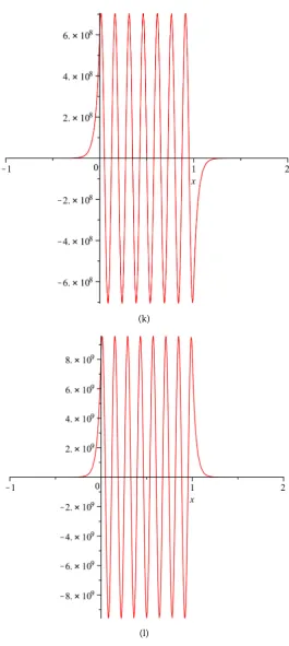
6π in a smaller rectangle. In Figure 2, we show graphs of eigenfunctions corresponding to positive eigenvalues of the problem (8)-(9) when 2

0 20π ,

q = and from this figure, we

estimate the upper bound of the Richardson number λ_{+, and the integers} n_R+ and

H

n+. We also show a typical behaviour of the real and imaginary parts of the non-real

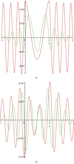
eigenfunctions corresponding to non-real eigenvalues of the problem (8)-(9) in Figure 1.

[image:8.595.196.552.91.599.2]

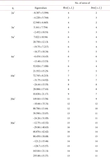
Table 1. Non-real eigenvalues obtained inside the rectangle E for some values of q0.

No. of zeros of

0

q Eigenvalues Reu x( ,λi) Imu x( ,λi)

2

2π −8.307 5.599i± 4 2 4.220 5.744i

− ± 3 3

12.940 6.665i± 4 2

2

3π 5.161 7.754i± 4 4 2.452 10.51i

− ± 5 3

2

5π 7.022 10.94i± 6 4 20.750 12.13i± 5 5

19.75 7.217i

− ± 6 4

16.37 10.34i

− ± 5 5

2

6π −6.434 14.43i± 6 6 13.40 13.53i

− ± 7 5

52.026 7.100i± 6 4 21.552 15.25i± 7 5

2

10π 72.745 8.215i± 7 7 31.75 14.92i

− ± 9 7

24.44 15.55i

− ± 8 8

28.886 17.61i± 8 8 10.838 21.17i± 9 7

2

20π 149.84 13.56i± 11 9 10.66 33.31i

− ± 12 12

88.706 13.44i± 12 10 39.590 33.07i± 13 11

24.26 31.05i

− ± 13 11

2

30π −12.75 43.52i± 15 15 29.86 40.63i

− ± 16 14

48.876±42.62i 16 14 88.450 18.68i± 15 15

121.2 15.46i

− ± 14 14

128.7 15.57i

− ± 15 13

163.04±21.11i 14 14 255.88 15.37i± 13 11

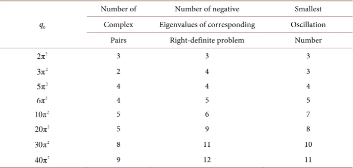
the real and imaginary parts of non-real eigenfunctions fails in the two-turning point case. Table 2 shows that the smallest number of zeros of the eigenfunctions corre- sponding to positive eigenvalues for each value of the parameter q0 considered, is two

[image:9.595.195.553.101.271.2]

Table 2. Comparing number of pairs of non-real eigenvalues with number of negative

eigenvalues of corresponding RDP.

0 q

Number of Number of negative Smallest Complex Eigenvalues of corresponding Oscillation

Pairs Right-definite problem Number

2

2π 3 3 3

2

3π 2 4 3

2

5π 4 4 4

2

6π 4 5 5

2

10π 5 6 7

2

20π 5 9 8

2

30π 8 11 10

2

40π 9 12 11

problem (8)-(9).

A closer look at Figure 2 shows that the smallest positive eigenvalue for this case is

1 61.02

λ ≈ _{with corresponding eigenfunction} u x₁

_{( )}

oscillating twelve times in the

interval. Furthermore, λ ≈2 119.62 and corresponding eigenfunction oscillating

eleven times in

(

−1, 2 .

)

The oscillation numbers decrease by one as the value of λ

increases until the fifth eigenvalue. From the sixth eigenvalue onwards the oscillation numbers increase by one as the value of λ _{increases and from the eleventh eigenvalue} (i.e., λ ≈11 778.48) onwards, each eigenfunction has a unique oscillation number. Since

11

λ has corresponding eigenfunction u11

( )

x oscillating thirteen times in

(

−1, 2

)

we

can say that for each n≥13 there is precisely one eigenfunction with n zeros in

(

−1, 2

)

and so n_H+ =13. Hence the correct notation is that ₁₁

( )

( )

,

R

n u x =u x λ+ and thus the Richardson number λ_{+ satisfies} 778.48

R

n

λ+<λ+ = . Another observation is that there is no positive eigenvalue with corresponding eigenfunction having less than eight zeros in

(

−1, 2

)

while for each n≥8, there is at least one eigenfunction having n zeros in

(

−1, 2

)

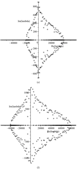
, hence we have that n_R+ =8.

Figure 3 gives the spectrum for larger values of q0 in the rectangle E. We see that

in each of the cases, the spectrum consists of a finite number of non-real eigenvalues and two infinite sequences of positive and negative eigenvalues.

3. Discussion and Conclusions

3.1. Discussion

From Figure 3, we see that the spectrum is made up of an infinite number of real eigenvalues and a finite number of non-real eigenvalues for each value of q0 con-

sidered. That the number of non-real eigenvalues of problem (8)-(9) is finite, is not a surprise because this is expected, by remark 1. It can be seen from the graphs of the eigenfunctions that generally oscillation numbers decrease as the parameter value increases, but then oscillations will stabilize and the usual oscillation theorem event- ually holds. This leads to the estimation of λ+_,

R

(a)

(c)

(e)

[image:12.595.244.506.73.650.2]

(f)

Figure 1. The case 2

0 30π

q = . Interlacing property for real and imaginary

parts of non-real eigenfunctions fails in the two turning points case. (a)

29.86 40.63i

λ= − + , (b) λ= −128.68 15.57i+ , (c) λ=163.04 21.11i+ , (d) 255.88 15.37i

(a)

(c)

(e)

(g)

(i)

(k)

[image:18.595.240.506.63.656.2]

(l)

Figure 2. Eigenfunctions corresponding to positive eigenvalues for the

case 2

0 20π

q = . (a) 61.01691, (b) 119.6179, (c) 159.1937, (d) 186.9206, (e)

(a)

(c)

(e)

[image:21.595.239.508.70.659.2]

(f)

Figure 3. Spectrum for the two-turning point case for selected values of q0.

(a) 2

0 20π

q = , (b) 2

0 30π

q = , (c) 2

0 40π

q = , (d) 2

0 500π

q = , (e) 2

0 4000π

q = ,

(f) 2

0 8000π

disconjugacy in the first and last intervals and many oscillations in the middle interval

( )

0,1 , since q0+λw>0 for all x∈

( )

0,1 because λ, ,w q0>0 in the interval.

However, for some values of λ _{a few oscillations are expected in the first and last} intervals. This is so because in some cases, q0 can be so large that q0−λ w>0. For

example in Figure 2, eigenfunctions corresponding to the first three positive eigenvalues have at least one zero in the first and third intervals.

Generally speaking, the number of non-real eigenvalues seems to increase with increasing q0. The number of pairs of distinct non-real eigenvalues of the problem

does not exceed the number of negative eigenvalues of the corresponding right-definite problem. For all values of q0 considered (cases where there are non-real eigenvalues),

the smallest oscillation number is 2 and so the problem does not have a positive eigenfunction in (−1,2). Furthermore, the real and imaginary parts of the non-real eigenfunctions do not interlace which is different from the results in the one turning point case considered by Richardson [4]. For larger values of q0, some non-real eigen-

functions vanish once in

(

−1, 2 ,

)

since the the real and imaginary parts of such

functions are both zero at x=0.5 (see for example, Figure 1(b), Figure 1(d), and Figure 1(f)). This was not one of the observation in the paper [18] in which we only considered generally smaller values of q0.

3.2. Conclusions

In this paper, we undertook a numerical study of the non-real eigenfunctions and eigenvalues of a non-definite Sturm-Liouville problem with two turning points, paral- leling the study in [7] in the case of one turning point. Our ultimate goal was to examine the behavior of the eigenfunctions, both real and non-real, of this non-definite Sturm-Liouville problem.

One of the interesting observations was that the zeros of the real and imaginary parts of a non-real eigenfunction interlace in some subintervals of

(

−1, 2

)

and not on the

whole interval, contrary to the results on the one turning point case covered in theorem 3. Whether this is an accident or a result of a more general yet unproven theorem, is unknown, but we conjecture that it is so and pose this as an open question for future research.

It is further observed that the complex eigenfunctions (corresponding to non-real eigenvalues) do not vanish in

(

−1, 2

)

, at least for smaller values of q0 considered in

this paper, while for some larger values of q0, there are cases in which the non-real

eigenfunctions vanish once in

(

−1, 2

)

. We note that this result seems to verify theorem

2 which indicates that if an eigenfunction of problem (8)-(9) has to vanish, it may do so at most once in the interval

(

−1, 2

)

, since in this case n=2. However, there is need to establish sufficient conditions for a non-real eigenfunction to vanish in an interval, say

( )

a b, . Thus, we have our second open question.

of the imaginary part of a non-real eigenfunction corresponding to a non-real eigen- value. Also this may be a consequence of a more general theorem which we don’t know, so then, we have a third interesting open question for future research.

Summing up, we mean that the research initiated in [18] and presented in detail in this paper has implied a number of new interesting open questions of both theoretical and practical importance.

Acknowledgements

The author wishes to thank Prof. Angelo B. Mingarelli (Carleton University, Ottawa, Canada), and Prof. Lars-Erik Persson (Luleå University of Technology) for reading through the manuscript and giving valuable suggestions and comments.

We also wish to thank the International Science Programme in mathematical sci- ences, Uppsala University, Sweden, and Luleå University of Technology, Sweden, for financial support which made this research possible.

Furthermore, we thank the careful referee for good suggestions and questions that improved the final version of this paper.

References

[1] Al-Gwaiz, M.A. (2008) Sturm-Liouville Theory and Its Applications. Springer-Verlag, London.

[2] Mingarelli, A.B. (1983) Volterra-Stieltjes Integral Equations and Generalised Ordinary Dif-ferential Expressions. Lecture Notes in Mathematics 989, Springer-Verlag, Berlin.

http://dx.doi.org/10.1007/BFb0070768

[3] Mingarelli, A.B. (1982) Indefinite Sturm-Liouville Problems. In: Everitt, W.N. and Sleeman, B.D., Eds., Ordinary and Partial Differential Equations, Springer-Verlag, Berlin, 519-528.

http://dx.doi.org/10.1007/BFb0065022

[4] Richardson, R.G.D. (1918) Contributions to the Study of Oscillation Properties of the Solu-tions of Linear Differential EquaSolu-tions of the Second Order. American Journal of Mathe-matics, 40, 283-316. http://dx.doi.org/10.2307/2370485

[5] Allrgretto, W. and Mingarelli, A.B. (1989) Boundary Problems of the Second Order with an Indefinite Weight Function. Journal für die reine und angewandte Mathematik, 398, 1-24. [6] Mingarelli, A.B. (1986) A Survey of the Regular Weighted Sturm-Liouville Problem: The

Non-Definite Case. Applied Differential Equations, World Scientific, Singapore, 109-137. [7] Atkinson, F.V. and Jabon, D. (1984) Indefinite Sturn-Liouville Problems. Proceeding of

1984 Workshop on Spectral Theory of Sturm-Liouville Differential Operators, Argon Na-tional Laboratory, 15 May-15 June 1984, 31-45.

[8] Kikonko, M. and Mingarelli, A.B. (2013) On Non-Definite Sturm-Liouville Problems with Two Turning Points. Journal of Applied Mathematics and Computing, 219, 9508-9515.

http://dx.doi.org/10.1016/j.amc.2013.03.025

[9] Qi, J. and Chen, S. (2014) A Priori Bounds and Existence of Non-Real Eigenvalues of Inde-finite Sturm-Liouville Problems. Journal of Spectral Theory, 4, 53-63.

http://dx.doi.org/10.4171/JST/61

31-61. http://dx.doi.org/10.1016/0022-0396(89)90112-5

[11] Haupt, O. (1915) Über eine methode zum beweise von oszillationstheoreme. Mathema-tische Annalen, 76, 67-104. http://dx.doi.org/10.1007/BF01458673

[12] Behrndt, J., Katatbeth, Q. and Trunk, C. (2009) Non-Real Eigenvalues of Singular Indefnite Sturm-Liouville Operators. Proceedings of the American Mathematical Society, 137, 3797- 3806. http://dx.doi.org/10.1090/S0002-9939-09-09964-X

[13] Mingarelli, A.B. (1988) Non-Real Eigenvalue Estimates for Boundary Problems Associated with Weighted Sturm-Liouville Equations. Proceeding of International Conference on Theory and Applications of Differential Equations, Columbus, 21-25 March 1988, 222-228. [14] Qi, J., Xie, B. and Chen, S. (2016) The Upper and Lower Bounds on Non-Real Eigenvalues

of Indefinite Sturm-Liouville. Proceedings of the American Mathematical Society, 144, 547- 559. http://dx.doi.org/10.1090/proc/12854

[15] Behrndt, J., Chen, S. and Qi, J. (2014) Estimates on the Non-Real Eigenvalues of Regular Indefnite Sturm-Liouville Problems. Proceedings of the Royal Society of Edinburgh Section A, 144, 1113-1126. http://dx.doi.org/10.1017/S0308210513001212

[16] Xie, B. and Qi, J. (2013) Non-Real Eigenvalues of Indefnite Sturm-Liouville Problems.

Journal of Differential Equations, 255, 2291-2301.

http://dx.doi.org/10.1016/j.jde.2013.06.013

[17] Behrndt, J., Philipp, F. and Trunk, C. (2013) Bounds on the Non-Real Spectrum of Diffe-rential Operators with Indefnite Weights. Mathematische Annalen, 357, 185-213.

http://dx.doi.org/10.1007/s00208-013-0904-7

[18] Kikonko, M. (2012) Non-Definite Sturm-Liouville Problems with Two Turning Points.

Proceeding of East African Universities Mathematics Programme (EAUMP) Conference, Arusha, 22 to 25 August 2012, 52-60.

Submit or recommend next manuscript to SCIRP and we will provide best service for you:

Accepting pre-submission inquiries through Email, Facebook, LinkedIn, Twitter, etc. A wide selection of journals (inclusive of 9 subjects, more than 200 journals)

Providing 24-hour high-quality service User-friendly online submission system Fair and swift peer-review system

Efficient typesetting and proofreading procedure

Display of the result of downloads and visits, as well as the number of cited articles Maximum dissemination of your research work