Risk components in UK cross sectional equities: evidence of regimes and overstated parametric estimates

Munich Personal RePEc Archive

Risk components in UK cross-sectional

equities: evidence of regimes and

overstated parametric estimates

Rossi, Francesco

30 November 2011

Modelling systematic and non-systematic risk in U.K. cross-sectional equities:

evidence of regimes and overstated parametric estimates

Francesco Rossi

UCD Michael Smurfit Graduate Business School

Banking & Finance

Dublin, Ireland

[email protected]

DUBLIN, IRELAND

NOVEMBER 2011 Abstract

We study the behavior and interaction of systematic and idiosyncratic components of risk in a

cross-section of U.K. stocks. We find no clear evidence of a trend in any component of total risk,

but we document different “regimes” in the behavior of each component of total risk, in their

correlation patterns and thus in their contribution to aggregate risk. Comparing parametric and

non-parametric estimates of residual risk, we find the former to significantly overstate

diversifiable risk, opposite to some previous findings for the U.S. market, with the difference

Contents

1. Introduction ...3

1.1 Modelling the behaviour and role of idiosyncratic risk ...3

1.2 Contribution ...5

2. Methodology and results ...5

2.1 Dataset ...5

2.2 Non-parametric volatility measures ...6

2.3 Comparison of parametric and non-parametric measures ... 13

3. Conclusions ... 18

1.

Introduction

1.1

Modelling the behaviour and role of idiosyncratic risk

Traditional asset pricing frameworks distinguish the determinants of the risk of assets between

systematic components, i.e. those driven by common, explicit risk factors, and “residual”,

“non-systematic” or “idiosyncratic” components. The idiosyncratic component can be thought of as

the component of returns that is specific of each single security – but also as the residual

component from a model that is by nature incomplete.

Within a broader stream of literature that looks to identify empirical pricing “anomalies”,

several researchers have studied the behaviour and role of the idiosyncratic component of

stock returns volatility, often documenting aggregate or cross-sectional effects partly

incompatible with the assumptions of traditional models. For instance, the CAPM assumption

that idiosyncratic risk should not be priced has been challenged both theoretically and

empirically, although with mixed results. But from a modelling standpoint, the behaviour of

idiosyncratic risk and its interaction with other risk sources is important for a number of

reasons. Firm-level volatility accounts for a large share - over sixty-percent according to some

estimates - of total volatility and volatility variation; in addition, asset holders and portfolio

managers are exposed to idiosyncratic risk because of portfolio or wealth constraints,

transaction costs, regulation, informational differences and explicit choice. As a result,

improving the knowledge of the determinants of such risk will bear consequence on asset

allocation decisions and from a risk-management standpoint improve the assessment of

portfolio risk exposures, in terms of breaking down the overall risk into factor exposures and

evaluating scenarios for the movement and correlation between them.

Idiosyncratic risk is defined as the risk that is unique to a specific firm, and it unobservable,

decomposition techniques to isolate it from systematic components of risk. Our analysis starts

from the results of papers such as Malkiel and Xu (1997), Campbell et al. (2001), Xu and

Malkiel (2003), that have measured and modelled idiosyncratic risk as part of an effort to

model the behaviour of total volatility, seen as the sum of market, sector and stock

components, revealing important features of the size, variation and trends of each component

that have important implication in a pricing framework. These papers using U.S. samples have

documented a strong correlation between the components, a particularly high variability of the

idiosyncratic one and its apparent upward trend - not accompanied by a rise in market

volatility. Although the finding of rising idiosyncratic risk has been questioned by more recent

papers (Bekaert, Hodrick, and Zhang (2008); Brandt, Brav, Graham, and Kumar (2010);

Bartram et al. (2009), Guo and Savickas (2008)) that have shown it is a product of a particular

sample, ending with the nineties, Campbell et al. (2001) also present evidence on the

characteristics and movement of the components of average volatility: firm-level volatility

accounts for the largest share of total volatility and volatility variation over time; the three

components of volatility move together and are countercyclical; market volatility tends to lead

the other volatility series. Moving away from U.S. samples, the results for international markets

are mixed. Bekaert et al. (2008) show that idiosyncratic risk has a large common component

across countries, which has gained importance over time. But the findings of Hamao et al.

(2003) for the post-crash Japanese market - a reduction in firm-level volatility in the context of

rising market volatility and equity co-movement – show clearly that the different micro and

1.2

Contribution

In our analysis of a U.K. sample, we apply the aggregate volatility decompositions of Malkiel

and Xu (1997) and Campbell et al. (2001), but we find no clear evidence of a trend in any

component of total risk; instead we find the idea of “regimes” emerging in Bekaert et al. (2008)

applicable and useful not only in modelling the pattern of each of the sub-components of total

risk, but also in modelling correlation patterns between each of them, and thus their

contribution to aggregate risk. This implies that the relative importance, variability and

co-variation of the components of total risk change significantly over time.

Comparing direct and indirect estimates of residual risk, we find the former to significantly

overstate diversifiable risk; this is the opposite of the findings of Xu and Malkiel (2003),

although they operate on a U.S. sample, use conditional estimates of both measures, and

obtain a moderate difference, while our difference is very large especially when we include the

industry component.

2.

Methodology and results

We estimate aggregate measures of volatility using both non-parametric and parametric

techniques.

2.1

Dataset

Our starting universe includes all stocks listed on the London stock exchange from January

1990 until December 2009, for which we collect monthly data from Datastream (prices,

returns, volume, outstanding shares and classification tags). A key issue emerging from the

literature on residual risk is the importance of controlling for the cross-sectional impact of

outliers, in the form of small and illiquid stocks. Bali et al. (2005) and Wei and Zhang (2005)

influenced by outliers. We deal with this issue, and with data-related problems in general,

using a combination of rigorous data-quality and investability filters, detailed fully in Rossi

(2011), including an in-depth cross-check and correction of the Datastream sample using a

second data source, Bloomberg. As a result, we are confident that our results are not

influenced to any significant degree by data errors or liquidity issues.

2.2

Non-parametric volatility measures

First, we compute the volatility of the market, as the standard deviation of the value-weighted

average of all single stock returns in our filtered sample1_{, over a twelve-month rolling window.}

Second, we calculate the value-weighted sum of the volatilities of all stocks over time; this

corresponds to the “aggregate” volatility measure of Malkiel and Xu (2003), is of course higher

than the market volatility due to the correlation effect, and can be viewed as the overall

volatility of a typical stock. Then we take the difference between the two measures to obtain the

portion of idiosyncratic volatility of the stocks in the index, which is diversified away in the

value-weighted portfolio. This idiosyncratic risk component is found to be trending up in Xu

and Malkiel (1997), Malkiel and Xu (2003) and Campbell et al. (2001) for a sample of U.S.

stocks; Campbell et al. (2001), for instance, report that while market volatility has no

significant trend, firm-level variance displays a large and significant positive trend, more than

doubling between 1962 and 1997, with a corresponding decrease in correlations and in the

explanatory power of the single factor model. But later studies, such as Bekaert et al. (2008),

have questioned the existence of such trend, showing it is highly dependent on the specific

sample cut-off; Frazzini and Marsh (2003) find no trend on the idiosyncratic volatility

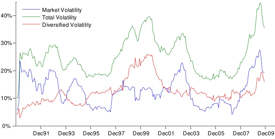
component for the U.K. market. In our sample, the existence of a trend is anything but evident,

with the idiosyncratic component oscillating around a level of 10%; graphical analysis points to

different “regimes” or periods of increased firm-specific risk, followed by phases of

normalization, implying that a trend could be detected if the end-point of a specific sample falls

during such episodes, but not otherwise. Two phases of marked increases in firm-level variance

can be observed in coincidence with the tech bubble and with the financial crisis at the end of

the sample. In contrast to the firm-specific component, the market component is much more

volatile around its mean, with multiple sharp increases corresponding to periods of turbulence

or recessions; the two components are comparable in average size, and one can graphically

spot that how they seem to move pretty independently of one another, often exhibiting a

negative correlation, except during the 2008 financial crisis. For example, it is evident that

while the volatility spikes of 1999 and 2002 are driven by only one component while the other

remains fairly stable, the 2008 spike is driven by increases in both components.

Dec91 Dec93 Dec95 Dec97 Dec99 Dec01 Dec03 Dec05 Dec07 Dec09 0%

10% 20% 30% 40%

Average Volatility Measures, %

Market Volatility Total Volatility Diversified Volatility

Figure 1 - Aggregate volatility measures, % - The figure shows Total, Market and Diversified aggregate

volatility, computed as in Malkiel and Xu (2003). The values are annualized, estimated with a rolling window of twelve

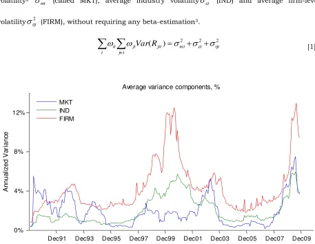
We then perform a second non-parametric variance decomposition using the methodology of

Campbell et al. (2001), decomposing aggregate variance into market, industry, and

idiosyncratic components. The average variance of a randomly drawn stock is split into market

volatility2 2

mt





volatility



2 2 2

)

(

i j

jt i

it



Var

R



















 [1]

Dec91 Dec93 Dec95 Dec97 Dec99 Dec01 Dec03 Dec05 Dec07 Dec09 0% 4% 8% 12% A n n u a li ze d V a ri a n ce

Average variance components, %

MKT IND FIRM

Figure 2 - Average variance components, %- The figure shows the components of the average variance of

a random stock: the market component (MKT), the industry-level (IND) and the firm-level component (FIRM). Data are

annualized and estimated with a rolling window of twelve monthly returns

The industry and firm components show a high degree of co-variation throughout the entire

sample. The market component, on the other hand, is fairly de-correlated with the other two at

least until the start of the last decade. Compared to the previous decomposition, which

separated systematic from the diversified component of volatility, this more granular

disaggregation into three components allows a better characterization of the volatility spike

corresponding to the 2008 financial crisis. Not only has the size of the increase in aggregate

total volatility been exceptional, but remarkably all three components moved up at the same

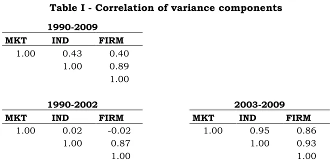
time, which had not been the case in the 1999 episode. Table I shows the correlation between

the three components of variance for the whole sample and for the sub-periods 1990-2002 and

2003-2009. While the correlation between the IND and the FIRM components remains always

very high, the correlation between the MKT component and the other two drops to zero to

slightly negative for the period up and including 2002, but becomes as high as 0.95 for the

second part of the sample from 2003 to 2009. To our knowledge, these distinctly different

correlation “regimes” have not been previously documented.

Table I - Correlation of variance components

1990-2009 MKT IND FIRM

1.00 0.43 0.40 1.00 0.89 1.00

1990-2002 2003-2009

MKT IND FIRM MKT IND FIRM

1.00 0.02 -0.02 1.00 0.95 0.86

1.00 0.87 1.00 0.93

1.00 1.00

We now turn to examine how important the three volatility components are relative to the total

volatility of an average firm, in terms of mean and variation. Campbell et al. (2001) had found

firm-level volatility to be on average the largest portion of total volatility, accounting for over

70%, followed by marked volatility at 16% and firm-level volatility at 12%. Or results, shown in

Table II, are broadly consistent with Campbell et al. (2001), although they paint a somewhat

more balanced picture: the largest component is indeed FIRM, which accounts on average for

over 50% of total variance, with the rest evenly split between MKT and IND. The importance of

the industry-specific component is higher in our sample. However, the most striking result is

that, if we split again the sample in two around 2002, the relative contributions to the average

total variance vary very little over the two selected sub-periods.

Table II - Decomposition of Mean of total variance, % values

MKT IND FIRM

1990-2009 0.23 0.25 0.52

1990-2002 0.23 0.25 0.53

2003-2009 0.24 0.24 0.52

Campbell et al. (2001) had shown, through a variance decomposition, that most of the

time-series variation in total volatility was due to variation in MKT and FIRM, with FIRM variance

and the covariation of MKT and FIRM being the two largest components; together they

accounted for about 60 percent of the total time-series variation in volatility, while the market

component alone contributed just by 15 percent. Relative to its mean, however, MKT showed

the greatest time-series variation, while the volatility of IND was more stable over time. To

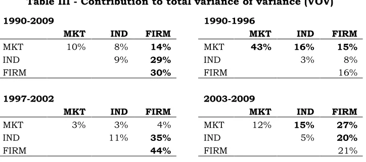
perform a decomposition4 _{of the variance of variance (VOV), we split our sample in three}

periods of roughly equal length: 1990-1996, 1997-2002 and 2003-2009. Table III shows the

4In this paragraph we are discussing the “variance of variance” (VOV), thus terminology becomes slightly cumbersome

contribution to total VOV by the three components and their covariance terms. Similar to the

results of Campbell et al. (2001), the variance of FIRM is often a key driver of total VOV, but in

fact we can identify distinctively different “regimes” corresponding to our sub-sample periods.

In the 1990-1996 period, MKT is the primary driver, accounting alone for 43% of total VOV,

and totalling 75% with the added impact of its covariation with IND and FIRM; this was a

period of fairly low aggregate volatility, the variability of which was thus driven by market-wide

movements, with no industry-specific shocks. During the following period, 1997-2002, total

VOV is instead driven almost entirely by FIRM (44%) and by its covariation with IND (35%),

while the importance of MKT is negligible. This period, leading to and including the tech bubble

and its eventual burst, captures a regime dominated by stock-specific and industry-specific

volatility. The final period, 2003-2009, shows a more balanced contribution, in line with the

high correlations between the three components documented in Table I: the co-variation terms

make up the bulk of total VOV.

Table III - Contribution to total variance of variance (VOV)

1990-2009 1990-1996

MKT IND FIRM MKT IND FIRM

MKT 10% 8% 14% MKT 43% 16% 15%

IND 9% 29% IND 3% 8%

FIRM 30% FIRM 16%

1997-2002 2003-2009

MKT IND FIRM MKT IND FIRM

MKT 3% 3% 4% MKT 12% 15% 27%

IND 11% 35% IND 5% 20%

FIRM 44% FIRM 21%

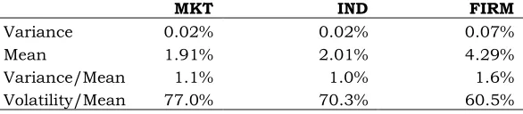
To describe the time-series variation of the variance components, we show in Table IV that

FIRM has the largest variance and mean, which explains its significant contribution to total

volatility; MKT and IND have lower values, similar to each other. Campbell et al. (2001) had

found MKT to have the highest variance relative to its mean; this is not true for our sample,

although both MKT and IND show a greater volatility relative to their means than FIRM5_.

Overall, we can say that the contribution of FIRM to total VOV is expected to be always high,

given its high mean and variance. The contribution of MKT and IND is more variable with time,

but we can state that the contribution of MKT is the least predictable, as it shows the weaker

correlation with the other two components and a high volatility around its mean; IND shows

instead a more slow-moving nature, and often mirrors FIRM, as can be seen easily in Figure 2.

Table IV - Time-series variation of variance components

MKT IND FIRM

Variance 0.02% 0.02% 0.07%

Mean 1.91% 2.01% 4.29%

Variance/Mean 1.1% 1.0% 1.6%

Volatility/Mean 77.0% 70.3% 60.5%

The Table shows the means, variance and volatility for the three components of total variance

Summarizing, we have the following results:

i. The correlation between the three components of total variance varies substantially over

time, although they tend to move together and experience periods of strongly positive

co-variation. The exception is the relationship between FIRM and IND, which is always very

strong: this implies that the joint contribution of the FIRM and IND (the stock-specific

and industry-specific components) to total variance is substantial, and very frequently a

large portion of that comes through the covariance terms. In contrast, the MKT

5 _{The inconsistency is only apparent here, as we are in fact showing that the results vary significantly with the selected}

component shows periods of high correlation with the other two components, but also

periods of very weak or near zero correlation

ii. In terms of relative contribution to total variance, FIRM explains on average (including the

impact of half of its covariance terms) 52% of the total, followed by IND and MKT with

28% and 21% respectively, roughly a quarter each. However, although those

contributions to the level of overall variance appear quite stable, looking at the drivers of

changes in volatility we find the contributions of each component to the variance of

variance to vary greatly in different sub-periods, identifying distinctly different regimes

iii. In terms of time-series variation, FIRM has the largest absolute variance and mean; yet

MKT and then IND show the greatest volatility relative to their means. The contribution of

FIRM to total variation is expected to be always high, while the share of MKT and IND

changes more over time. Correlation analysis tells us that the contribution of MKT in

particular is more uncertain and difficult to predict, as it is more weakly correlated with

the other two components

2.3

Comparison of parametric and non-parametric measures

2.3.1Parametric estimation of risk factor loadings and residual risk

We obtain parametric estimates of systematic and idiosyncratic risk exposures running two

alternative regressions

ri,t= αi,t + βi,t rM,t + εi,t [2]

ri,t= αi,t + βi,t rM,t + hi,t HMLt + si,t SMBt + εi,t [3]

The first one is the market model, while the second one controls for the two additional

points, expanding from a minimum of 12 observations6_{. The monthly returns for the HML}

factor is obtained from Kenneth R. French’s website7_{, while we compute the SMB factor by}

sorting our filtered sample into ten size deciles.

We collect the series of β, s, h, estimated from the above regressions as our (contemporaneous)

estimates of systematic risk exposures. We also collect the series of the residuals εt to generate

estimates of the idiosyncratic risk σ2_{. We then build} σ2 _{using the two alternative approaches}

most common in the literature:

i. as the rolling standard deviation of the (rolling) series of εt over the 24 months window8

ii. fitting a GARCH(1,1) model to the series of the variance of εt over the 24 months window,

and generating on each period a forecast for the conditional volatility of εt . The model is

σt2= k + g σt-12+ a εt-1 [4]

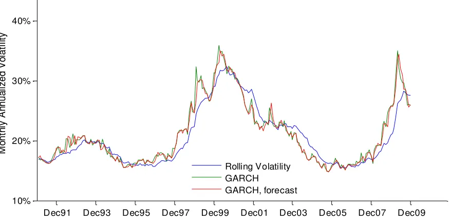
The results of the two estimation procedures are shown in Figure 3, where we display

aggregate, value-weighted measures of σt2across the entire sample.

6 _{Empirical methods to obtain estimates of risk premia vary, and should be considered carefully for their econometric}

implications. For insance, OLS estimation over a rolling window assumes there is sufficient structure on the temporal variation in the parameters that OLS estimates may reasonably be interpreted as estimates of their mean values

7 _{http://mba.tuck.dartmouth.edu/pages/faculty/ken.french/data_library.html#International}

8 _{The most commonly used procedure to estimate idiosyncratic volatility is to use the standard deviation of residuals}

Dec91 Dec93 Dec95 Dec97 Dec99 Dec01 Dec03 Dec05 Dec07 Dec09 10%

20% 30% 40%

M

o

n

th

ly

A

n

n

u

a

lize

d

V

o

la

ti

lit

y

Aggregate Average Idiosyncratic Volatility, %

Rolling Volatility GARCH

GARCH, forecast

Figure 3 - Average idiosyncratic volatility, % - The figure shows average (value-weighted) idiosyncratic

volatility measures, in annualized % terms, built from the residuals series from the cross-sectional single factor model regression. For each month t, we show three alternative volatility estimates: the simple standard deviation of the residual series, the conditional GARCH(1,1) volatility, and the conditional GARCH(1,1) volatility forecast for month t+1

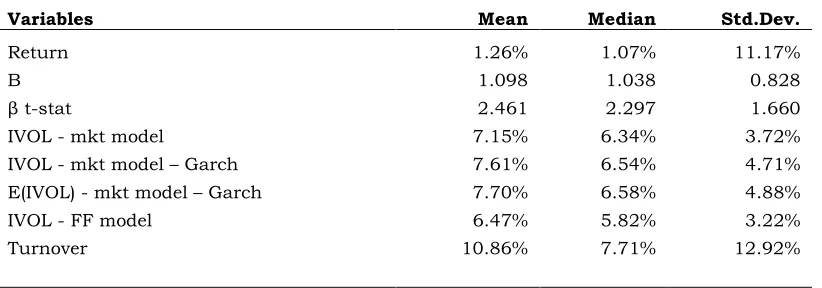
Having obtained estimates of risk-factor exposures, Table V presents the variable descriptive

Table V - Variable descriptive statistics for the pooled sample

Variables Mean Median Std.Dev.

Return 1.26% 1.07% 11.17%

Β 1.098 1.038 0.828

β t-stat 2.461 2.297 1.660

IVOL - mkt model 7.15% 6.34% 3.72%

IVOL - mkt model – Garch 7.61% 6.54% 4.71%

E(IVOL) - mkt model – Garch 7.70% 6.58% 4.88%

IVOL - FF model 6.47% 5.82% 3.22%

Turnover 10.86% 7.71% 12.92%

Descriptive statistics for the pooled sample - monthly data from January 1990 to December 2009.

The “Mean” values are not market-value weighted but equally weighted. The first 12 months (January-December 1990) have been excluded to allow for estimation of betas and volatility terms.

“IVOL” is the cross-sectional idiosyncratic volatility, obtained regressing stock returns on a constant and the market return; “IVOL - mkt model”, “IVOL - mkt model – Garch” and “E(IVOL) - mkt model - Garch” are obtained from the residuals of a single factor model regression, and are respectively a rolling 24-month average, a GARCH(1,1) term and its 1-period-ahead forecast. “IVOL - FF model” is

instead obtained from a 24-month average of residuals from a Fama-French regression.

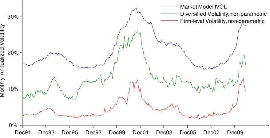
2.3.2Comparing parametric and non-parametric residual risk measures

Comparing the average measure of residual risk built from the factor model regression

residuals to the non-parametric estimates of residual risk of Section 2.2, as we do in Figure 4

and Table VI, it is evident how either the single factor model or the Fama-French model do a

pretty poor job in capturing all sources of systematic risk. The single factor model parametric

measure is on average 1.6 and up to 2.5 times higher that the “diversified“ non-parametric

measure (5.4 and up to 9 times higher than the “firm-level” measure built using the

methodology of Campbell et al. (2001), which obtains as the component of average total risk

not driven by market or industry risk). The comparison does not improve much using the

parametric measure obtained from the Fama-French regression, as shown in Table VI . In

annualized volatility terms, this translates into a gap of 7.6% (16%) on average - and up to 15%

implies that idiosyncratic risk measures built from standard regressions reflect a substantial

amount of risk that, in reality, is systematic. It is worth noting that this result is the opposite

of the findings of Xu and Malkiel (2003), although they employ conditional estimates of both

measures, their sample is U.S.-based and their difference between the two measures is smaller

(the non-parametric measure is 0.1 times larger on average).

Dec91 Dec93 Dec95 Dec97 Dec99 Dec01 Dec03 Dec05 Dec07 Dec09 0% 10% 20% 30% M o n th ly A n n u a li ze d V o la ti lit y

Parametric and non-parametric measures of Idiosyncratic Volatility, %

Market Model IVOL

Diversified Volatility, non parametric Firm-level Volatility, non-parametric

Figure 4 - Parametric and non-parametric measures of Idiosyncratic Volatility, % - The

figure shows in blue the average (value-weighted) idiosyncratic volatility from the single factor model cross-sectional regression, together with the two non-parametric measures described in section Error! Reference source not found.:

Table VI - Ratio of parametric estimates of average idiosyncratic volatility to

non-parametric estimates of diversified or stock-specific risk

Parametric Estimates

Single Factor Model

Fama-French Model

Non-parametric measures

Max

Average

Max

Average

Malkiel's "diversified" volatility

2.43

1.67

2.19

1.51

Campbell's firm-specific volatility

9.05

5.43

8.46

4.94

The table shows the ratio of parametric estimates of average idiosyncratic volatility (obtained with a single factor model regression or with a Fama-French regression) to non-parametric estimates of diversified or stock-specific

risk (the average “diversified” volatility built as in Xu and Malkiel (2003) or the firm-specific average volatility as in Campbell et al. (2001) )

The extent of this over-estimation of the idiosyncratic component, of extremely large

proportions in comparison to the measure of Campbell et al. (2001), suggests considerable

caution towards results claiming to find a significant cross-sectional price for residual risk;

they likely point to structural issues with the pricing model or with the systematic factor

exposures estimation procedure.

3.

Conclusions

We have reviewed and expanded some results on the behaviour of idiosyncratic risk and its

interaction with systematic components of total risk. Our analysis of a U.K. sample has

confirmed the idea that the components of total risk, including the idiosyncratic one, exhibit no

time trend, but we show that they are subject to regimes affecting substantially the pattern of

their movement and correlation and thus their contribution to aggregate risk. This implies that

the relative importance, variability and co-variation of the components of total risk change

significantly over time. We would stress two results. First, the Industry component and the

firm-specific (or idiosyncratic) component are always highly correlated, while the market

contribution of the three components to total risk is quite stable (with the firm-specific

component accounting for over half of the total), the drivers of changes in total risk are not. We

obtain another important result comparing parametric and non-parametric estimates of

residual risk, and finding that parametric measures greatly overstate diversifiable risk; this

implies that a large portion of parametric estimates of residual risk are likely to be in fact

References

Amihud, Yakov, 2002, Illiquidity and stock returns: cross-section and time-series effects,

Journal of Financial Markets, 5, 31-56.

Ang, Andrew, Robert J. Hodrick, Yuhang Xing, and Xiaoyan Zhang, 2009, High idiosyncratic

volatility and low returns: International and further U.S. Evidence, Journal of Financial

Economics 91, 1-23.

Ang, Andrew, Robert J. Hodrick, Xing Yuhang, and Zhang Xiaoyan, 2006, The cross-section of

volatility and expected returns, Journal of Finance 61, 259-299.

Arena, Matteo P., K. S. Haggard, and Xuemin Sterling Yan, 2008, Price momentum and

idiosyncratic volatility, FinancialReview 43, 159-190.

Bali, Turan G., Nusret Cakici, Zhang Zhe, and Y. A. N. Xuemin, 2005, Does idiosyncratic risk

really matter?, Journal of Finance 60, 905-929.

Bartram, Söhnke M., Gregory Brown and Rene M. Stulz, 2009, Why Do Foreign Firms Have

Less Idiosyncratic Risk than U.S. Firms?, Working Paper.

Basu, Devraj, and Lionel Martellini, 2007, Total volatility and the cross section of expected

stock returns, EFMA Working Paper, Draft.

Bekaert, Geert, Campbell R. Harvey and Christian Lundblad, 2007, Liquidity and Expected

Returns: Lessons from Emerging Markets, Review of Financial Studies 20, 1783-1831.

Bekaert, Geert, Robert J. Hodrick, and Xiaoyan Zhang, 2008, Is there a trend in idiosyncratic

volatility?, Working Paper.

Boyer, Brian H., Todd Mitton, and Keith Vorkink, 2008, Expected idiosyncratic skewness,

Brandt, Michael W., Alon Brav, John R. Graham and Alok Kumar, 2010, The Idiosyncratic

Volatility Puzzle: Time Trend or Speculative Episodes?, Review of Financial Studies 23,

863-899.

Brockman, Paul, Maria Gabriela Schutte and Wayne Yu, 2009, Is Idiosyncratic Risk Priced?

The International Evidence, Working Paper.

Campbell, John Y., Martin Lettau, Burton G. Malkiel, and Xu Yexiao, 2001, Have individual

stocks become more volatile? An empirical exploration of idiosyncratic risk, Journal of

Finance 56, 1-43.

Carhart, Mark M., 1997, On persistence in mutual fund performance, Journal of Finance 52,

57-82.

Chen, Joseph S., 2002, Intertemporal capm and the cross-section of stock returns, SSRN

eLibrary.

Chua, Choong Tze, Jeremy Goh, and Zhe Zhang, 2006, Idiosyncratic volatility matters for the

cross-section of returns - in more ways than one!, Working Paper.

Cremers, K. J. Martijn, and Jianping Mei, 2002, A new approach to the duo-factor-model of

return and volume, New York University, Working Paper.

Cremers, K. J. Martijn, and Jianping Mei, 2007, Turning over turnover, The Review of Financial

Studies 20, 1749.

Epstein, Larry G., and Martin Schneider, 2008, Ambiguity, information quality, and asset

pricing, Journal of Finance 63, 197-228.

Fama, Eugene F. 1968a, Risk, Return and Equilibrium, Center for Mathematical Studies in

Business and Economics, University of Chicago, Report No. 6831.

Fama, Eugene F., 1968b, Risk, Return, and Equilibrium: Some Clarifying Comment, Journal of

Fama, Eugene F., and Kenneth R. French, 1992. The cross-section of expected stock returns.

Journal of Finance 48, 427–465.

Fama, Eugene F., and Kenneth R. French, 2008, Dissecting anomalies, Journal of Finance 63,

1653-1678.

Frazzini, A., and L. Marsh, 2003, “Idiosyncratic Volatility in the US and UK Equity Markets,”

Unpublished Working Paper, Yale University.

French, K., G. Schwert, and R. Stambaugh, 1987, Expected stock returns and volatility,

Journal of Financial Economics.

Fu, Fangjian, 2009, Idiosyncratic risk and the cross-section of expected stock returns, Journal

of Financial Economics 91, 24-37.

Garcia, René, Daniel Mantilla-Garcia and Lionel Martellini, 2009, Idiosyncratic Risk and the

Cross-Section of Realized Returns: Reconciling the Aggregate Returns, Working Paper.

Guo, Hui and Robert Savickas, 2008, Average Idiosyncratic Volatility in G7 Countries, Review

of Financial Studies 21, 1259-1296.

Guo, Hui, and Robert Savickas, 2004, Idiosyncratic volatility, stock market volatility, and

expected stock returns, Working Paper.

Hamao, Yasushi, Jianping Mei, and Yexiao Xu, 2003, Idiosyncratic risk and the creative

destruction in Japan, NBER Working Paper.

He, Zhongzhi, Sahn-Wook Huh and Bong-Soo Lee, 2008, Is Dynamic Factors and Asset Pricing,

Working Paper.

Ince, Ozgur S., and Burt R. Porter, 2006, Individual equity return data from Thomson

Datastream: handle with care!, Journal of Financial Research 29, 1475-6803.

Jacobs, Kris, and Kevin Q. Wang, 2004, Idiosyncratic consumption risk and the cross section

Jegadeesh, Narasimhan, and Sheridan Titman, 2001, Profitability of momentum strategies: An

evaluation of alternative explanations, Journal of Finance 56, 699-720.

Jensen, Michael C., Fischer Black and Myron Scholes, 1972, The Capital Asset Pricing Model:

Some Empirical Tests, Studies in the theory of capital markets 81, 79-121.

Lehmann, Bruce N., 1986, Residual risk revisited, NBER Working Paper.

Lehmann, Bruce N., 1992, Empirical testing of asset pricing models, NBER Working Paper.

Li, Xiafei, Joëlle Miffre, Chris Brooks, and Niall O'Sullivan, 2008, Momentum profits and

time-varying unsystematic risk, Journal of Banking & Finance 32, 541-558.

Malkiel, B. G., and Yexiao Xu, 2002, Idiosyncratic risk and security returns, Working Paper.

Malkiel, Burton G., and Yexiao Xu, 1997, Risk and return revisited, Journal of Portfolio

Management 23, 9.

Merton, Robert C., 1987, A simple model of capital market equilibrium with incomplete

information, Journal of Finance 42, 483-510.

Rossi, Francesco, 2011, U.K. cross-sectional equity data: do not trust the dataset! The case for

robust investability filters, MPRA

Ruan, Tony, Quian Sun an Yexiao Xu, 2010, When Does Idiosyncratic Risk Really Matter?,

Working Paper.

Spiegel, Matthew, and Xiatong Wang, 2005, Cross-sectional variation in stock returns:

Liquidity and idiosyncratic risk, Yale School of Management, Working Paper.

Wei, Steven X., and Chu Zhang, 2005, Idiosyncratic risk does not matter: A re-examination of

the relationship between average returns and average volatilities, Journal of Banking &

Finance 29, 603–621

Xu, Yexiao, and Burton G. Malkiel, 2003, Investigating the behavior of idiosyncratic volatility,