Improvement of Liver Segmentation by Combining High
Order Statistical Texture Features with Anatomical
Structural Features
Suhuai Luo1, Xuechen Li1, Jiaming Li2 1The University of Newcastle, Australia
2The CSIRO ICT Centre, Australia Email: [email protected]
Received 2013
ABSTRACT
Automatic segmentation of liver in medical images is challenging on the aspects of accuracy, automation and robust-ness. A crucial stage of the liver segmentation is the selection of the image features for the segmentation. This paper presents an accurate liver segmentation algorithm. The approach starts with a texture analysis which results in an opti-mal set of texture features including high order statistical texture features and anatomical structural features. Then, it creates liver distribution image by classifying the original image pixelwisely using support vector machines. Lastly, it uses a group of morphological operations to locate the liver organ accurately in the image. The novelty of the approach is resided in the fact that the features are so selected that both local and global texture distributions are considered, which is important in liver organ segmentation where neighbouring tissues and organs have similar greyscale distribu-tions. Experiment results of liver segmentation on CT images using the proposed method are presented with perform-ance validation and discussion.
Keywords: Liver Segmentation; Texture Feature; Support Vector machine; Morphological Operation
1. Introduction
Automatic and accurate liver segmentation in medical images such as computed tomography (CT) and magnetic resonance imaging (MRI) is one of the most important concentrations in medical image processing. Segmenta-tion of liver from its surrounding organs and tissues are a crucial yet very difficult task in building a surgical plan-ning system for liver transplantation and resection. This is because the boundary between the liver and its neighbouring structures such as the heart is sometimes barely noticeable in CT images, and the liver is nonrigid in shape and variant in position.
Various algorithms have been proposed to deal with liver segmentation, including live wire-based, gray level- based, neural networks-based, model fitting-based, prob-abilistic atlas-based, graph cut, deformable model-based, level set-based, and machine learning-based [1-9]. Al- though much progress has been achieved in recent years, challenges remain on the aspects of segmentation accu-racy, robustness and automation.
This paper presents an automatic liver segmentation by combining high order statistical texture features with anatomical structural features. Section two describes the algorithm in detail, including texture analysis, liver
dis-tribution image calculation with support vector machines, and liver organ localization with a group of morphologi-cal operations. Section three gives the details of the liver segmentation experiment on CT images, including the experiment setting, performance validation and discus-sion, and future work in the area.
2. The Approach
The proposed automatic liver segmentation in CT images consists of three major processes as shown in Figure 1,
including texture analysis, liver distribution image cal-culation, and liver organ localization.
Abdominal CT images
Texture feature analysis
Liver distribution image calculation
Liver region localization
[image:2.595.81.262.66.317.2]Segmented liver organ
Figure 1. The diagram of the proposed automatic liver seg-mentation.
2.1. Texture Feature Analysis
In abdominal CT images, liver shows similar grey scales and textures to its neighbouring structures such as heart and stomach. Therefore, three important considerations are taken in developing the proposed algorithm. First, liver segmentation based on greyscale parameters alone is not sufficient; second, high order texture parameters can better deal with liver segmentation; lastly, optimal liver segmentation can be achieved when global ana-tomical structural features are used.
Since homogeneity and consistency characterize liver segmentation where multiple slices and different patients are dealt with, texture features are considered. Textures are complex visual patterns that are composed of entities or subpatterns that have characteristic brightness, colour, slope, size, etc. [10]. It can be regarded as a similarity grouping in an image. Methods of texture analysis can be broadly classified into four categories, including: struc-tural approach, which represents texture by defined primitives; statistical approach, which represents texture by non-deterministic properties that govern the distribu-tions and reladistribu-tionships between grey levels of an image; model-based approach, which uses fractal and stochastic models to interpret image texture; and transform ap-proach, which represents image in a space where texture is well characterised. The statistical approach and the transform approach are investigated and adopted in the proposed segmentation method, mainly based on the facts that the statistical approach has the advantage of representing texture inexplicitly and the transform ap-proach has the advantage of representing texture at vari-ous scales.
2.1.1. Grey Level Co-occurrence Matrix and Haralick Texture Descriptors
In characterising the distribution and relationship of pix-els, i.e. texture, in a grey scale image, the joint probabil-ity distribution of pairs of pixels is used. It is defined as the co-occurrence matrix. Its normalised form is noted as Cij(d, θ) [11].
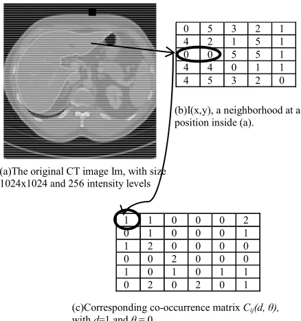
In an image Im of size H by W pixels and with G in-tensity levels, for every pixel centered on a neighborhood I(x,y) of size N by N, Cij(d, θ) is defined as the total numbers of times that, within the N by N neighborhood:
[image:2.595.312.531.473.707.2]I(x1,y1) = i and I(x1+dcosθ, y1+dsinθ) = j (1) where x1 = 0, 1, …, N-1, is the row number in the neighborhood ; y1= 0, 1, …, N-1, is the column number in the neighborhood; i = 0,1,…,G-1, is the row number in the co-occurrence matrix ; j = 0,1,…,G-1, is the column number in the co-occurrence matrix; d = 1,…,N-1, is the displacement distance along θ; θ = 0°, 45°, 90°, 135°, is the angle between the pair.
Figure 2 illustrates the calculation of Cij(d, θ) at a pixel in an abdominal CT image. The co-occurrence ma-trix is square and has a size G, which is the intensity lev-el in original image. Note that in Figure 2 (b), for the
sake of easy description, the maximal intensity value is supposed to be 5, much less than that of original liver CT image. For a normalised CT image, the maximal inten-sity value is usually 255. In the figure, the curved line connecting (b) and (c) shows how C00(1, 0) is calculated: for d = 1 and θ = 0, within the 5 by 5 neighborhood, the total number of times that a pair of 0-value pixels ap-pears is one, so C00(1, 0) = 1.
1 1 0 0 0 2 0 1 0 0 0 1 1 2 0 0 0 0 0 0 2 0 0 0 1 0 1 0 1 1 0 2 0 2 0 1
0 5 3 2 1 4 2 1 5 1 0 0 5 5 1 4 4 0 1 1 4 5 3 2 0
(a)The original CT image Im, with size 1024x1024 and 256 intensity levels
(b)I(x,y), a neighborhood at a position inside (a).
(c)Corresponding co-occurrence matrix Cij(d, θ),
with d=1 and θ= 0.
The co-occurrence matrix basically keeps track of all the pixel-pair counts. It is also called spatial dependence matrix. Since representing an image with its co-occur- rence matrix will result in much more data (e.g., for an image of size 1024 by 1024 pixels and with 256 intensity levels, the co-occurrence matrix will be of size 256 by 256 by 1024 by 1024), a set of features with much less size yet reflecting the co-occurrence characters was pro-posed, known as Haralick texture descriptors [11]. The nine Haralick texture descriptors can be defined and cal-culated as below.
Entropy: measures the randomness of gray-level dis-tribution: lj G i G j ij C C log
(2)
Energy: measures the occurrence of repeated pairs:
Gi G
j ij
C2 (3)
Contrast: measures the local contrast:
2
( )
G G
lj i j
ij C
(4)Sum Average: measures the average of the gray-level:
1 ( 2 G G lj lj i j
iC jC
) (5)Variance: measures the variation of gray-level distri-bution:
2
1 (( ) ( ) )
2
G G
r lj c lj
i j
i C j C
2 (6)Correlation: measures a correlation of pixel pairs:
2 2
( )( )
G G
r c
i j r c
i j
Cij(7)
Maximum Probability (MP): gives the most predomi-nant pixel pair:
,
, G G
ij i j
Max C (8)
Inverse Difference Moment (IDM): measures the smoothness: 2 1 G G ij i j C i j
(9)Cluster Tendency: measures the grouping of pixels that have similar gray-level values:
2 (
G G
r c
i j
i j
) Cij (10)where Cij is the normalised co-occurrence matrix with
displacement distance d and angle θ; r, c,
2
r
, and 2
c
are the means and variance of row and column in Cij(d,θ).
2.1.2. Wavelet Coefficients
Wavelet coefficients are the output of wavelet transform (WT) [12] which is the decomposition of a signal into a set of basis functions consisting of contractions, expan-sions and translations of a mother wavelet .
The wavelet transform of a signal f(x) is defined as
* 1 ,
( , ) , u s ( ) s (t u)
Wf u s f f t dt
s
(11)where the mother wavelet is a zero average function, centered around zero with a finite energy. The family of vectors is obtained by translations and dilatations of the mother wavelet: , 1 ( ) ( ) u s t u t s s
(12)
In image processing applications, the wavelet trans-form is usually computed with dyadic wavelet transtrans-form which is implemented by filter banks. The filtering is done along both row and column with pairs of lowpass filter and highpass filter [12]. Figure 3 illustrates the
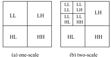
process of deriving wavelet coefficients for an image using the dyadic wavelet transform. Figure 3 (a) gives a
one-scale wavelet decomposition result which has four blocks of components: LL is the downsampling of the lowpass filtering along both row and column, LH is the downsampling of the lowpass filtering along row and highpass filtering along column, HL is the downsampling of the highpass filtering along row and lowpass filtering along column, and HH is the downsampling of the high-pass filtering along both row and column. Such filtering or decomposition can be done further on LL, resulting a two-scale wavelet decomposition of an image as shown in Figure 3 (b). Note that the number of total wavelet
coefficients equals to the number of the pixels in the im-age, no matter being a one-scale decomposition or two- scale decomposition. In general, there will be 4 + 3* (S - 1) blocks for an S-scale decomposition.
LL LH
HL HH HL HH
LH LL LL LL LH LL HL LL HH
[image:3.595.62.289.251.658.2](a) one-scale (b) two-scale
[image:3.595.331.513.604.697.2]Comparing to other transforms such as Fourier [13] and Gabor [14], Wavelet transform has two advantages in segmentation application. One is that it can represent textures at the most suitable scale by varying the spatial resolution. The other is that wavelets best suit for texture analysis in a specific application can be chosen because of a wide range of choices for the wavelet function.
2.1.3. Combining High Order Statistical Texture Features with Anatomical Structural Features
As discussed before, the grey level co-occurrence matrix and related Haralick texture descriptors are second-order statistical texture features. They have the advantages of describing the statistic relationships among neighboring pixels. However, in practical segmentation applications, they are confined by two factors – small local range cov-erage and huge computation load. The small local range coverage is the fact that the co-occurrence matrix is cal-culated within a neighboring of N by N pixels. N is usu-ally a single digit value, e.g., 5, considering the computa-tion load. To consider the statistical texture representa-tions for an image, the computation load is huge. For example, for an image of size 1024 by 1024 pixels and with 256 intensity levels, if three kinds of pixel-pairs are considered (i.e., the displacement distances d = 1, 2, 3), and only one direction is considered (i.e., angle between the pair θ =0), 3 × 9 × 1024 × 1024 Haralick texture descriptors will be calculated, with each calculation be-ing propotional to the task of derivbe-ing the co-occurrence matrix of size 256 by 256.
Wavelet coefficients can compensate Haralick de-scriptors in specifying texture, by providing features to describe anatomical structure at a large scope with vari-ous resolutions. For example, for a WT of 3 scales and filter length 9, a coefficient in the lowest resolution block can represent the texture of 8 × 9 pixels, which will well cover the important anatomical structure around liver.
Therefore, to fully take the advantages of high order statistical texture features and anatomical structural fea-tures, both Haralick texture descriptors and WT coeffi-cients are used as the inputs to liver distribution image calculation stage.
2.2. Liver Distribution Image Calculation
The liver distribution image of an abdominal CT image is a binary image. In the distribution image, the values of the pixels are one if the pixels have the most possibility of being liver, whereas the values of the other pixels are zero. Support vector machines (SVMs) [15] are imple-mented as classifier to pixelwisely derive the distribution image. SVMs are a set of discriminative classifiers which are defined by an optimal separating hyperplane. View-ing input data as two sets of vectors in an n-dimensional space, the hyperplane will maximize the margin between
the two data sets.
The SVMs classifiers are built in a training process. In the process, assume the training set is {(xi,yi), i =1,2,…l}, where xi is the input with xi∈Rn, yi is the output with yi∈ RR={-1,+1}, and l is the number of input samples. Then an optimal hyperplane in canonical form must satisfy the following constraints:
( )x b 0
(13) where b∈R, is a normal vector, and ( )x is an inner product induced feature map that maps the input space into a high dimension linear space.
SVMs convert the task of finding the optimal hyper-plane into a task of quadratic programming problem as:
2 1 2
1
min( l i)
i
C
subject to
( ) 1 , { 1
i i i i
y x b y ,1} (14) Applying Lagrange multipliers, the optimal quadratic programming problem can be solved as the following dual optimal problem:
1 2
1 1 1
max{l i l j i j i j ( , )}i
i i j
y y K x x
ji
subject to
1
0 i , and l i 0
i
C y
(15)where i is support value, the xi corresponding to
0iC is support vector (SV), and the xi corre-sponding to 0iC is normal support vector (NSV).
1 [ (
NSV
i j
i j j i N
x NSV x SV
b y y K x
, )]xj (16)where NNSV is the number of NSV, K x x( , )i j is kernel function. Typical kernel functions are linear, polynomial, radial basis function, and sigmoid.
The training process will derive i, b, and K x x( , )i j . Then the SVM as a classifier can classify any input data x with the following classify function:
1
( ) {l i i ( , )i }
i
f x sign y K x x b
(17)2.3. Liver Region Localization
The liver distribution image derived with SVMs is a bi-nary image. It can indicate most of the liver correctly.
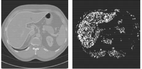
Figure 4 illustrates one such example, where the left is
Figure 4. An example of liver distribution image left: an original image; right: output of SVMs.
Observing the distribution image, two issues need be tackled. One is that the classification is not perfect, re-sulting misclassified pixels both within the liver and out-side the liver. The other is that the shape and spatial in-formation is not considered, making the classification sensitive to the noise produced by the misclassified pix-els. Therefore, a set of binary morphological operations [16] is specifically designed to get the delineation of the liver out of the distribution image.
The morphological operation starts with dilate and erode on the distribution image to get connected regions. Morphologic operations are described by the shape and size of the structural element used. Considering both the anatomical structural knowledge of the abdomen and the CT image resolutions, a square structural element with a diameter of 6 pixels is chosen. The second stage of the morphological operation is to further purify the outcome of the first stage. This includes: to retain the largest ob-ject; to remove the pixels that are liver yet are misclassi-fied as non-liver using hole filling operation; and to de-lete the spurs and smooth the contour along edges with erode and dilate operation.
3. Experiments and Discussions
The proposed automatic liver segmentation algorithm was applied to human abdominal CT images obtained from [17]. All the images were enhanced with contrast agent and scanned in the central venous phase on a vari-ety of scanners ranging from 4 to 16 and 64 detector rows. All the data were acquired in transversal direction. The pixel spacing varied between 0.55 and 0.80 mm, the inter-slice distance varied from 1 to 3 mm. In the ex-periments, eight images from one subject were chosen as training set to train the SVM classifier, and testing set were the images from another subject.
Segmentation performance validation was done by comparing the automatic segmentation results with the benchmark provided by the data supplier. Three metrics are designed to evaluate the algorithm as below.
False positive volume fraction (FPVF)
FPVF is defined as the amount of the pixels that are
falsely classified as the liver by the proposed method, as a fraction of the total amount of pixels that are identified as the liver in the benchmark. It can be expressed as:
SVM man
man
L L
FPVF L
where Lman denotes the total amount of pixels that are identified as the liver by benchmark. LSVM denotes the total amount of the pixels that are classified by the pro-posed method as the liver. |LSVM- Lman | is the set differ-ence between LSVM and Lman.
False negative volume fraction (FNVF)
FNVF is defined as the amount of the pixels that are falsely classified by the proposed method as non-liver, as a fraction of the total amount of pixels that are identified as the non-liver in the benchmark. It can be expressed as:
man SVM
man NL NL FNVF
NL
where NLman denotes the total amount of pixels that are identified as non-liver in the benchmark. NLSVM denotes the total amount of the pixels that are classified by the proposed method as non-liver. |NLman-NLSVM| is the set difference between NLman and NLSVM.
True positive volume fraction (TPVF)
TPVF is defined as the amount of the pixels that are classified as liver by both the proposed method and in the benchmark, as a fraction of the total amount of pixels that are identified as the liver in the benchmark. It can be expressed as:
proposed man
man
L L
TPVF
L
where Lproposed denotes the total amount of the pixels that are classified as the liver by the proposed method.
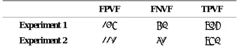
The procedure of the experiments are so designed that the performance comparison is done between the method using high order statistical texture features only and the method using both high order statistical texture features and anatomical structural features. Two experiments had been done. In experiment 1, nine Haralick texture de-scriptors (as defined in equations 2 to 10) were used to derive the liver distribution image. Where d = 2, θ = 0, and the intensity was normalized to 256 levels. In ex-periment 2, in addition to the nine Haralick texture de-scriptors, Wavelet coefficients were used. Where scale number S = 3. In both the experiments, the parameters for SVMs are the same, including using a polynomial kernel function.
Table 1 shows the performance comparison of the two
Table 1. Performance metrics (%) of the two experiments.
FPVF FNVF TPVF
Experiment 1 14.7 6.3 93.8
Experiment 2 11.1 5.1 97.3
statistical texture features only are used. The perform-ance improvement is across all the metrics, with about four percent improvement on TPVF.
4. Conclusions
This paper presents an accurate liver segmentation algo-rithm. The main focus of the discussion is how to im-prove segmentation performance by selecting most suit-able image features. There are three major steps in the proposed method, including texture analysis which re-sults in a suitable set of texture features, calculation of liver distribution image using support vector machines, and accurate liver organ localization using a group of morphological operations to locate the liver organ. The novelty of the approach is resided in the fact that the features are so selected that both local and global texture distributions are considered. Out of detailed methodology description and segmentation experiments, it has shown that the proposed method can accurately segment liver in CT image, achieving as high as 97.3% on true positive volume fraction.
REFERENCES
[1] A. M. Mharib, A. R. Ramli, S. Mashohor and R. B. Mah-mood, “Survey on liver CT image segmentation methods”,
Artificial Intelligence Review, Vol. 37, No. 2, 2012, pp. 83-95.doi:10.1007/s10462-011-9220-3
[2] H. Bourquain, et al., “Hepavision2—A Software Assis-tant for Preoperative Planning in Living Related Liver Transplantation and Oncologic Liver Surgery,” Computer Assisted Radiology&Surgery, 2002, pp. 341-346. [3] H. P. Meinzer, M. Thorn and C. Cardenas,
“Computer-ized Planning of Liver Surgery: An Overview,” Com-puters and Graphics, Vol. 26, No. 4, 2002, pp. 569-576. [4] P. Campadelli, E. Casiraghi and A. Esposito, “Liver
Seg-mentation from Computed Tomography Scans: A Survey and a New Algorithm,” Artificial Intelligence in Medicine, Vol. 45, No. 2-3, 2009, pp. 185-196.
doi:10.1016/j.artmed.2008.07.020
[5] S. Luo, Q. Hu, X. He, J. Li, S. J. Jin, S. Chalup and M. Park, “Automatic Liver Parenchyma Segmentation from Abdominal CT Images Using Support Vector Machines,”
2009 IEEE/CME Int. Conf on Complex Medical
Engi-neering, April 9-11, 2009, Tempe, USA, paper 10071. [6] V. Pamulapati, A. Venkatesan, B. J. Wood and M. G.
Linguraru, “Liver Segmental Anatomy and Analysis from Vessel and Tumor Segmentation via Optimized Graph Cuts,” MICCAI'11 Proceedings of the Third international conference on Abdominal Imaging: Computational and Clinical Applications, 2011, pp. 189-197.
[7] T. Dima and J. Domingo, “A Local Level Set Method for Liver Segmentation in Functional MR Imaging,” IEEE Nuclear Science Symposium Conference Record, 2011, pp. 3158-3161.
[8] J. Lu, L. Shi, M. Deng, S. C. H. Yu and P. A. Heng, “An Interactive Approach to Liver Segmentation in CT Based on Deformable Model Integrated with Attractor Force,”
Machine Learning and Cybernetics (ICMLC) 2011, pp. 1660-1665.
[9] Y. Zhao, Y. Zan, X. Wang and G. Li, “Fuzzy C-means Clustering-Based Multilayer Perceptron Neural Network for Liver CT Images Automatic Segmentation,” Control and Decision Conference (CCDC) 2010, pp. 3423-3427. [10] A. Materka and M. Strzelecki, “Texture Analysis
Meth-ods - a Review,” Technical Report, Technical University of Lodz, Institute of Electronics, 1998.
[11] R. M. Haralick, “Statistical and Structural Approaches to Texture,” Proceedings of the IEEE, Vol. 67, No. 5, 1979, 786-804.doi:10.1109/PROC.1979.11328
[12] S. Mallat, “Multifrequency Channel Decomposition of Images and Wavelet Models”, IEEE Trans. Acoustic, Speech and Signal Processing, Vol. 37, No. 12, 1989, pp. 2091-2110.
[13] A. Rosenfeld and J. Weszka, “Picture Recognition in Digital Pattern Recognition,”K. Fu (Ed.), Springer-Verlag, 1980, pp. 135-166.
doi:10.1007/978-3-642-67740-3_5
[14] J. Daugman, “Uncertainty Relation for Resolution in Space, Spatial Frequency and Orientation Optimised by Two-Dimensional Visual Cortical Filters,” Journal of the Optical Society of America, Vol. 2, 1985, pp. 1160-1169. doi;10.1364/JOSAA.2.001160
[15] N. Cristianini and J. Shawe-Taylor, “An Introduction to Support Vector Machines and Other Kernel-based Learn-ing Methods,” Cambridge University Press, ISBN 0521780195, 2000.doi:10.1017/CBO9780511801389 [16] J. Serra, “Image Analysis and Mathematical
Morphol-ogy,” Theoretical Advances, New York: Academic, Vol. 2, 1998.