SORA Dynamics and Control System Studies Using Mean Value Neutron Kinetics Equations EUR 4408

¡iff1·'

»Rift

w

E U R 4 4 0 8 e

m

WW

U « . «jfr ι

EUROPEAN ATOMIC ENERGY COMMUNITY ­

SORA DYNAMICS AND CONTROL SYSTEM

STUDIES USING MEAN­VALUE

I ' r f S f f l p

NEUTRON KINETICS EQUATIONS

by

R. ARHAN

«H

J

ΑΙ

iffPif

™IH!røli

mim

Joint Nuclear Research Genter Ispra Establishment - Italy Reactor Physics Department

Research Reactors

>3¡V *]

Smf*

W&ÊËàh

mm

• f*îT"· F#

'töSiffiift

iPM

LEGAL NOTICE

#*5

■*«i

This document was prepared under the sponsorship of the Commission of the European Communities. "lüír"',!

Neither the Commission of the European Communities, its contractors

nor anj* person acting on their behalf : ,*. ,\

make any warranty or representation, express or implied, with respect to the accuracy, completeness or usefulness of the information con­ tained in this document, or t h a t the use of any information, apparatus, method or process disclosed in this document may not infringe privately owned rights; or

assume any liability with respect to the use of, or for damages resulting from the use of any information, apparatus, method or process disclosed in this document.

This report is on sale at the addresses listed on cover pat^e 4

a t the price of F F 13.80 F B 125.­ DM 9.20 Lit. 1 560 Fl. 9 ,

'àmiú

\SÆ

W h e n o r d e r i n g , p l e a s e q u o t e t h e E U R n u m b e r a n d t h e title, w h i c h a r e i n d i c a t e d on t h e cover of e a c h r e p o r t .

I i l i

Printed by Guyot, s.a.

Brussels, January 1970

il'«I«

P*1 k*' · m k I ^ H H | i lit''·

ΜΨ-

Mmm mm^mmk

his document was reproduced on the basis of the best available copy,

EUR 4 4 0 8 e

EUROPEAN ATOMIC ENERGY COMMUNITY - EURATOM

SORA DYNAMICS AND CONTROL SYSTEM

STUDIES USING MEAN-VALUE

NEUTRON KINETICS EQUATIONS

by

R. ARHAN

1970

Joint Nuclear Research Center Ispra Establishment - Italy Reactor Physics Department

A B S T R A C T

The study described in this report deals with dynamics and control of the pulsed fast reactor SORA. It is based on a set of equations for mean-value neutron kinetics. A simulation of the complete set of equations, including thermal reactivity feed-back, is performed. As results, the reactor responses to perturbations of reactivity, inlet coolant temperature and coolant velocity are shown. Control rod malfunctions are investigated; a start-up procedure is proposed. A fast control system is synthesized.

KEYWORDS

SORA

REACTIVITY NEUTRONS

KINETIC EQUATIONS DISTURBANCES

COOLANTS TEMPERATURE VELOCITY

3

-TABLE OP CONTENTS

1. Introduction

2. Basic Equations for Description of the Reactor 2.1 Core kinetics - Conversion to power

2.2 Reactor thermal description 2.3 Reactivity feedback

2.4 Summary of equations

3. Simulation of the Uncontrolled Reactor 4. Startup Procedure

5. Linearized Reactor Description 6. Fast Control System

6.1 Closing the loop directly

6.2 First improvement of the fast control system perfor­ mances

6.3 Second improvement of the fast control system performances

6.4 Basic set of equations for the controlled reactor

7. Malfunctions 8. Conclusion

Appendix 1 - Derivation of numerical values for a steady state condition at power

Appendix 2 - Derivation of numerical values for subcriticai steady state condition

Appendix 3 - Reactor period. Nomenclature

- 5

50RA DYNAMICS AND CONTROL SYSTEM STUDIES USING MEAN-VALUE NEUTRON KINETICS EQUATIONS^ .»)

I. INTRODUCTION

The SORA reactor is a fas-t reactor periodically wised by reactivity variations designed as a neutron source for re­

search in neutron physics. The reactor design and experimental use have been described in several meetings, notably at Karls­ ruhe in 1965 (Ref. 6), at Santa Fe in 1967 (Ref. 7) and at Albuquerque in 1969 (Ref. 4).

The study described in the report was performed in the

year 1968 at the request of the SORA Project to answer questions which the project designers had about the reactor dynamics and control.

Mean-value neutron kinetics equations are used for this study. A set of equations for the reactor mean temperatures is used

for the calculation of thermal reactivity feedback.

A simulation of the complete set of equations is performed using the digital computer IBM 360/6 5. As results, the reactor responses to perturbations of reactivity, inlet coolant tem­ perature, and coolant velocity are shown. Also a start-up pro­ cedure is proposed. Control rod malfunctions occurring in the uncontrolled reactor are also investigated.

In a classical manner, the set of equations is linearized for small deviations from pulsed steady state to obtain a reactor transfer function which is used for the synthesis of the fast control system. This fast control system is then in­ troduced as a control loop around the reactor. The whole system is then simulated and checked against typical perturbations of reactivity, inlet coolant temperature and coolant velocity.

I wish to acknowledge the help and the interesting suggestions of Mr. Larrimore throughout this study.

2. Basic Equations for Description of the Reactor

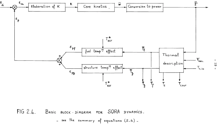
A block-diagram for dynamics of the uncontrolled reactor is shown in figure 2. See also the list of symbols at the end of this report. Three parts may be seen in this block diagram:

- core kinetics and conversion to power - thermal description

- reactivity feedback.

Three inputs are considered for this system:

- external reactivity ( <c )

- inlet coolant temperature (T · ) ^ c, in - coolant velocity (V , ) .

J cool

The three most important outputs (from dynamics point of view) are shown:

- power (P)

- fuel temperature (T~)

- structure temperature (T ).

Also available from the set of equations that we will use are a number of other parameters such as fission rate, outlet coolant temperature, internal reactivities from fuel and structure. For reasons of clarity all of these narameters were not shown in Fig. 2 .

£ . .— t o t a c r e a c t i v i t y £ , o l 4./c ^x

enfernox reactiVity

^

o d

d

- O

-d

Γ

CORE KIM Ε Τ ICS AND

C O N V E R S I O N TO POWER

tuet t e ™ b e r a t u r e ejrect

s t r u c t , t e m p e r a t u r e ePPect

REACTIVITY FEEDBACK

τ„

T H E R M A L I N S C R I P T I O N ^

Y

I

- a

1

8 ­

2.1 Core kinetics ­ Conversion to power

The kinetic theory of a periodically pulsed reactor was estab­

lished by Bondarenko and Staviskii (Ref.1). Later on,extensive

kinetic studies were performed at Ispra, namely by' Blässer,

Misenta and Raievski (Ref.2). The neeessary elements for a

clear understanding of the present report will be found in

the survey paper of Larrimore (Ref. 3 ) .

Since our main purpose was to get a good approximation for the

reactor transients and a reference design for control systems,

we decided to use "mean power kinetics" in a point reactor model

for such a work. By "mean power kinetics" we mean the time be­

haviour of the average values over a period of the power and pre­

cursor concentrations for times long compared to the pulse period,

In analogy with the multiplication factor for a stationary (non

pulsed) reactor, a multiplication factor K is here defined,

based (Ref. 2) on production and destruction of delayed neutron

precursors:

K" Precursor Production During Period

( 2 1 1 )

Precursor Decay During Period

\ ■*■■*■ J

with K = 1 for pulsed steady­state operation. This multiplication

factor, also called "pulsed multiplication coefficient" may

be

expressed as:

K

M

f

-L·

(2­1­2)

o

where M and e are functions of the r e a c t i v i t y l e v e l i n the

r e a c t o r . In Figure 2­1

a p l o t (Ref. 4) of K versus peak prompt

reactivity e · c a l c u l a t e d for the SORA r e a c t o r .

i s shown. The

r e p r e s e n t e d curve was f i t t e d a s :

K = 0,229 + 8,80 e

+ 0,0176 e

m

(2­1­3)

Now, s i n c e the p r e c u r s o r production during a period i s

ßvwT

and the p r e c u r s o r decay during the same time i n t e r v a l i s

Σλ­C.T

i

i t r e s u l t s d i r e c t l y from (2­1­1) t h a t the mean f i s s i o n r a t e i s :

w * ξ — ( ζ λ . δ . + S ) ( 2 - 1 - 4 )

βν i i i °

o

N)

i*.

u

1.2

5: _0.6

0.4

0.2

■100

MULTIPLICATION

FACTOR Κ

I

VERSUS

/

P L A K P K O M P ' I

K b A c n v i i Y ; é

/

-I I I I , I I I I I I I I

/ I

/ I

/ I

/

I

ι ι ι u

■so O 50 Smo 100

PEAK PROMPT REACTIVITY, €m (/>cn>)

10

dC.

d T = ß . ν₁ w

λ

Α

Equations (2-1-2) to (2-1-5) describe completely the r e a c t o r

k i n e t i c s . The corresponding r e a c t o r power i s s t r a i g h t forwardly

o b t a i n a b l e from the mean f i s s i o n rate w a s :

Ρ - —

■Γ — rt

c

( 2 - 1 - 6 ) .

We will write finally the complete and practical set of

equations for kinetics:

K =

w =

dC.

1

d t

Ρ =

0 , 2 2 9 + 8 , 8 0 em + 0 , 0 1 7 6 e 4 1 4 0 €m m

- — (Σ λ .C. + S )

βν i χ χ °

β± V w - λ ^

w

cf

(2­1)

2.2 Reactor thermal description

A simple mathematical model (Ref. 5) for the reactor thermal

description has been developped in collaboration with the SORA

Project, which expresses the mean fuel and structure temperatures

in terms of the power, the inlet coolant temperature and the

coolant velocity. These mean temperatures are used for the cal­

culation of thermal reactivity feedback.

The SORA reactor core consists of a bundle of approximately 116

fuel rods (Ref. 6 and 7). Assuming a uniform radial power gene­

ration and neglecting the heat flow in the vertical direction, a

temperature distribution such as shown in Fig. 2­2 may be defined

for any element, which enables us to calculate mean temperatures

for fuel, bond­clad, and coolant. The heat exchange coefficients,

calculated from these mean temperatures, are assumed to hold in

11

-Q

<C _)

O

+

O ζ

o

CÛ

t-z

<

_J

o o

CJ

r*

12

£z2zli_§Î˧ÉZzËΧîê_ÎËîïîEêî!§iHrË_aiËÏli5HÎè2SËi_!!?

.aG_Î

.5i

E£I!ËHE£Ë_ÎËËË_£igHr

._i::;2_)_

2­2­1­1. Temperature distribution in fuel. Mean fuel tem­

perature T~.

Assuming a uniform volume heat source q*', and k~ independent of

the temperature, the temperature distribution in a fuel element

is a solution of:

q* + kf V2Tf = 0.

Neglecting heat flow in the axial direction, this may be written

as:

τ '

ÏÏ7

Integrating once:

rdT­ q" ,r

d (-ΈΓΪ

= -

'

dTf

( — τ - = 0 at r = 0)

dr '

dTf

ÏÏF"

Integrating again:

ƒ

_Sk"

Tf(r)

rdr

q" r Tf(r) - Tf s

4 k„ _rf

The mean fuel temperature is defined as:

.r >

ƒ r

Tf(r)

.

Tfs

Tf - Tfs

2v rdr

­ 13

q ' 2

Tf " Tfs ­ Bk^ rf ·

Introducing finally the average power generation in fuel per 2 m

unit of length q = irr. q , we obtain:

q

f 8irkf f s *

2­2­1­2. Temperature distribution in bond­clad. Mean structure

temperature Τ .

For the purpose of this study the bond and clad are combined

into a single region. Due to the small thickness, one may write

directly (see figure 2­2):

q"

Tfs " Tgs = kg" ^ro " rf)

where qM is the average power per unit area. Introducing the

average power generation per unit of length q = 2 ir r~q" ,

we get:

q

Tfs " Tgs = 2π rfkg ^ro " rf '

The mean bond­clad or structure temperature is then defined as:

T

g ­ V

\

<

f

­ V ' ■ *«.

ττγι

f ^

'

T„ = τ. - i (τ. - τ )

=

i

-

-¡Λ-

(

° "

) .

^g = xtB - ? v±fs ­ xg s; = Afe ­ T7T _r.

g xf

2­2­1­3» Temperature distribution in the coolant. Mean coolant

temperature(or coolant temperature at half height of

core) Τ .

We assume the coolant temperature increases linearly from the

inlet to the outlet so that the mean coolant temperature is the

coolant temperature at half height of core. Following this

­ 14

q"

τ

where h„ is the heat transfer coefficient between clad and

coolant and a" the average power per unit area. Introducing

once again the average power generation per unit of length we

obtain:

q

τ ­ τ

2­2­2^ Stead^_state_heat_transf£r_£££ffÌ£ÌE2^E

From the previous equations we derive heat exchange coefficients

related to the characteristic temperatures T­, T , and T .

i g c

2 ­ 2 ­ 2 ­ 1 . Fuel to clad heat t r a n s f e r c o e f f i c i e n t hp

We have found :

_ q

T

f "

f s

BFÎÇ

q ro ~ rf Tf s ­ Tg = 4 IT kg ( ϊ~~ } '

Defining the heat t r a n s f e r coefficient h h

Fs q

we obtain:

r s Tf - T

h 1

Fs ' Λ « r - rf

1 ' f o f %

wnq

τττ;

r

2-2-2-2. Clad to coolant heat transfer coefficient q r

-Γ-Τ - -Γ-Τ = * ( — =■ )

g gs 4 w kg

Φ _ Φ = _

gs c 2ir r^h

rf

15

Defining the heat transfer coefficient h as:

h

S C m _rp

i t i s found:

h

1 _{/ o}r _ ­ r _{xf N J}

(~ 7 7 ~ } + 2TT r 3 "

4 7T k Γ » c ιι i -ρΛΧ-ρ

2­2­3^_Heat_balance_equations Fuel heat balance e q u a t i o n :

dT­

C

f d~r =

­

F s

f ­ V

'

(2­2­3­1)

Bond­clad or s t r u c t u r e heat balance e q u a t i o n : df

f­ = h,, (T­ ­ Τ ) ­ h n (Τ ­ Τ ) (2­2­3­2)

g dt Fs f g sc v g c

Coolant heat balance equation:

dT

LC

c

-a =

sc W

­

c(

c,out­

c,in)

(2­2­3­3­)

Tc - \ iTc,in+ Tc,out)· (2­2­3­4)

Assuming no time lag exists between Τ and Τ due to the small

g c

heat capacity of the coolant, equation (2­2­3­3) may be turned into:

Lhsc W = V Cc ^Tc,out­Tc,in) ' (2­2­3­5)

Equations (2­2­3­4) and (2­2­3­5) are then used to express Τ

and Τ . in terms of Τ and Τ . :

c,out g c,m

T

c = ­ ^ C ¡ — ·

\ *

li

c,in

<

­

­3­6>

1+ — 14­

16 'c, out 1 + 2VC Lh sc

τ β

-1­

1 + 2VC

c

L ho „

sc 2VC

c

sc

Τ

"c,m (2­2­3­7)

Eliminating finally Tc between (2­2­3­6) and (2­2­3­2), we get

for the structure heat balance equation:

dT

'g T Î =

Fs

f V

-SC /sr Lh

1 + sc 2VC.

(T„ - Τ , J

g c, m ' (2­2­3­8)

2­2­4i_Summar^_of_equations_for_the_rea^

Results (2­2­3­1), (2­2­3­8), (2­2­3­7) and (2­2­3­4) describe

the reactor from a thermal point of view. For clarity, we rewrite

here these results:

dTf

Cf dt~

dT

c

üg dt

Τ c, out Τ c ­ = = =

nL * P^ > ­ hFs

hFs <Tf ­

Τ + ­

c, m

1

2 uc , i n τ ì

V

1

2 2VC

i C

Lh r

SC

+ Τ 4

c, oui

CTf

­

3 Γ. f Φ Φ Ì

L hs c u g Χο,ίη;

+ 2VC

c

Cf Φ ì

g c, in;

.)

(2-2 )

2-3» Reactivity feedback

17

-The temperature coefficients of reactivity in SORA have

been calculated to be negative, which simplifies considerably all problems of control. The temperature effect is split

into two parts: the fuel temperature coefficient e - (in­ cluding fuel axial expansion and Doppler effect) and the structure temperature coefficient

turai expansion) so that:

e (including radial struc-Pg

V

=

ep g

€P =

_ * . af( Tf - TR E F)

ag( Tg - T REF)

e Pf + eP g

(2-3)

with a~ and α negative

2-4 Summary of equations

Equations for kinetics, thermal description, and feedback

reactivity are rewritten below. (See Fig. 2-4 for the relative block diagram.)

€, = input reactivity signal

e = total feedback reactivity signal * = total reactivity = e, + e . _{m J d ρ}

Κ = 0 . 2 2 9 + 8 . 8 0 e „ + 0 . 0 1 7 6 e4 1 4 0 em

m

w = K_ _βν

( \ \ c

s

)

d Ci

dT"

18 ­

d Τ f C

f d t p P ( t ) ­ hF s( Tf ­ Tg:

d Τ C — ¿

­ g d t hFs <T

f - V "

se Lh 1 + s e

(T ­ T . ) g c , i n ' 2VC

T

c , o u t Τ +

e , m 2 VC 1 +

(τ - τ . )

sc

(2-4)

:p f

—■ ( τ + τ )

2 c , i n c , o u t of ( Tf ­ T |E F )

' P S

«g <T

f -

W

ψ

M

rfr

Core kinetics w Conversion t o jiower

Τ

fuel temf>- e f f e c t

s t r u c t u r e t e r v i b ^ effect

X

*

T'

Tf

» t

L

T

T hervmoX

d e s c r u b t i o n

»

f

<

X

COOL· T

C , I M

<X3

FIG 2 - ¿ .

BLOCK - DiAGRAM

FOR SORA DYNAMICS.

-20

3. Simulation of the Uncontrolled Reactor

The simulation of the uncontrolled reactor was based on the set of equations (2-4). The use of a digital computer rather than an analog one was chosen mainly for the following reasons:

noise and thermal drift eliminated, easy calculation of K( e ),

amplitude scale unlimited. Therefore, the simulation consists of an iterative integration of the set of equations (2-4). Ve used the program SAHYB-2, developped at CETIS: this program was specially developped to meet the requirements of simulation on digital computers (Ref. 9).

It must be noted, however, that an iterative integration by means of a digital computer implies a cumulative error (as time goes on) on the integrated values. But this error may be kept

as low as desired by introducing the requested specifications into the program.

We first simulated the effects of:

- a change in reactivity,

- a change in coolant velocity, and - a change in inlet coolant temperature

on the uncontrolled reactor. These changes were introduced as step functions with the reactor assumed to be stabilized at power 600 kW. The relative initial conditions were calculated from the set of equations (2-4) for the steady-state condition 600 kW.

In Fig. 3*1 "the response to a step of reactivity of 5 pern is shown: the power jumps immediately by about 100 kW from the initial level 600 kW, which is characteristic of the kinetics of such a reactor (see equation 2-1-4); the power then stabilizes at about 30 kW above the initial level with a time constant of approximately 1 second.

ΔΡ(Μ) êj (rcm)

200

•igO 460

W

120

100

80

60

í.0

20

i d

ΔΡ"

[S3

h-»

I

Time (secondi)

1.5 2.5 3.5 «.5

RESPONSE TO A CHANGE ON REACTIVITY

( UN CONTROLLED REACTO R )

\,.°C APftw)

200

180

« 0

ftO

Ai/O

•loo

!0

ίο

AO

20

0 10

(0

50

AO

30

2o

■

·» '

0

ΔΤ

1.5 2.5

RESPONSE TO A CHANGE ON INLET COOLANT TEMPERATURE

( U N C O N T R O L L E D R E A C T O R )

3.5"

FIG. 5-2

T i m e ( seconds)

- 24

In Fig. 3-2, is plotted the power response to a negative step of 10°C on the inlet coolant temperature. The power stabilizes at about 70 kW from the initial level.

Finally, in Fig. 3-3 the power response to a positive step of 0,25 m/s in the coolant velocity is plotted. This results in a power increase of about 10 kW.

In the two last cases, the power level increases due to the fact that the considered perturbations reduce the reactor temperature

4. Startup Procedure

Simulating the set of equations (2-4) permits to> define:

- a procedure for approach to criticality (K = 1 )

- a procedure for bringing the reactor up to power 600 kW.

These procedures are intended as typical insertion rate curves for the uncontrolled reactor (no control, no scram system) and may be considered as the optimum insertion rates meeting the following specifications:

*

- start from subcriticai steady state

- approach to criticality as quick as possible

- period TR always £ 30 seconds

R άψ

dT

The insertion rates as shown in figure 4 have been found by. successively trying numerical values as slopes for f Although these results were derived empirically, they give a good first

approximation to an optimal startup procedure based on the previous specifications.

Some conclusions coming from this first approach are:

a) The approach to criticality must be performed very slowly:

the reactivity insertion must be held in the order of 0,1 pcm/s if the period has to be kept > 30 s. With this condition,

AP(lcW) V (cm/s)

20

•it

Ί2

ï - 300

200

•100

V

A?

1.5 2.5 5.5

RESPONSE TO A CHANGE ON COOLANT VELOCITY

(UNCONTROLLED REACTOR)

FIG. 3-5

lime ( secondi )

4.5

to

­ 27

the power level at criticality is reasonably high, that is in

the order of 150 mW.

b) The time for bringing the reactor up to power (600 kW) lies

in the order of 1000 seconds. This time seems to be the

minimum required for starting up to power with the imposed

safety condition on the period.

5. Linearized Reactor Description

A linearized reactor description is derived in this section

which leads to a transfer function for the whole reactor ­ in­

cluding kinetics, thermal description and feedback reactivity.

In a successive step comparisons are made, on the basis of the

reactor response to perturbations, between the set of non­linear

equations (2­4) and the derived transfer functions.

5­1 Derivation of transfer functions

We start with the set of equations (2­4) and consider small

deviations from the pulsed steady state.

5­1.zli_5Ëï!iY§îi2î}_2i_§_Îî!§BËÎe.£_ÎHB£ii2îi_£2r_£2ï!e.z^iîlËii£§

Assuming the reactor is at steady state at a certain power level,

we will denote by e the e value such that K( e ) = 1

( e = 9 1 , 1 pern) and consider small reactivity derivations

Δ? from this value. Then:

K

('mo

* m ) "

^ J = Ae

.(dT­)

mo which gives the following transfer function:

Α

< · > - ( Ι τ — )

·*<>>

V ΠΙ ¿ς

mo

AK(s) = 3,1745 ' 10"2-Ae m( s ) with Ae expressed in pern.

28

steady state

dC

Ko = 1'

10

dt 0

K

w = _2 ( Σ.λ .C.+S )

o ^ ι ι ι o;

dC.

1 0

dt

=

λ .c

small deviation

from

steady state

Κ + ΔΚ

W Q + Δνν = _ o _ _ r ­ , λ ι( ο .ο + A C i) + S0 d_/7T

dt ( Ci o+ A Ci) = ^ (wo + ¿ w ) - ^ ( Ï Ï ^ ûCi) Δ Κ

The s e c o n d ­ o r d e r t e r m Σλ.ΔΟ­ i s n e g l e c t e d . S i n c e a t s t e a d y /9v i

dC.

1 0

s t a t e Κ = 1 a n d «, = 0 , one o b t a i n s :

Δ ν ν _ _ ^ Σ λ àc.+ w AK

^v i i i o

d t ( A Ci) = ^ i v A w - λί A Ci

This set of equations is Laplace-transformed on both sides;

eliminating AC-(s) the following transfer function is obtained:

A w (s ) AK(s)

w

1-Σ

i

1_ S+ λ·

In turns, this result is approximated by a one-precursor group model as:

A,w s

ΔΚ (s w s + λ (see Ref. 10)

Introducing finally power instead of fission rate, we obtain the following transfer function relating the power variations

ΔΡ to the reactivity variations Ae :

° m

29

The n u m e r i c a l v a l u e chosen f o r λ i s 0 . 0 8 sec . Then, f o r t h e 600 kW power s t e a d y s t a t e , t h i s g i v e s :

AP

Ae 1,524

12,5 s + 1

m

Δ Ρ expressed in kW

Ae expressed in pern

(5­1­1)

5­2~2:L_Derivation_of_a_transfer_function

Assuming a constant velocity for the coolant, the set of equa­

tions (2­2) consists of linear differential equations and may be

directly Laplace­transformed. Since the mean fuel temperature

and the mean structure temperature are of main interest, we will

establish the results for these two temperatures only,

h

( s Cg+ hF s+ ~~

sc

Δ Τ , =

1 + sc _2VC

h™ h . <R Fs se

'

Lh7

1 + se 2VC

ΔΤ

c. m

s CoC + s

hF sCg + ( hF s+ ­ T h T — ) Cf

1 + _2"VC" se

+ hF s h_Lh s c

-" 1 + se

2vc"

h

phF s Δ Ρ + sc (sC­ + h „ ) Δ Τ

1 +

LK V Ö Wf T " F s

sc

2vc~

c, in

ΔΤ = g

s C~C + s

h sc

hFsCg + ( hF s+ ­

1 +

) C

l +

sc

J

2VC

IF

1 + _2~VC" sc

30

A Tf( s )

Δ T ( s )

A ( s )

BTÏÏ7

D ( s )

**<«> - H f l

( 5 - 1 - 2 )

A P ( s ) + UU ' ΔΤ _ ( s )

Bis _{c, m}

w h e r e : ( e x p r e s s i n g power i n kW and t e m p e r a t u r e i n C) h

A ( s ) = ( s Cg + hp s + se

Lh )

1 + s e 2VC

A ( s ) = 0 , 2 2 s + 2 , 9 8

B ( s ) = s C^.C + s h­™ C + ( h „ + F s g F s

sc__N ρ F s s e

Lh _; Uf i + Lh

1 + se

2VC 1 + 2VC. s e

B ( s ) = 3 , 1 1 7 s¿ + 4 5 , 1 7 6 s + 1 6 , 1 7 4

C ( s ) =

h­o h _{F s s e}

Lh 1 + se

2VC

C ( s ) = 1 6 , 1 7 4

D ( s ) = ρ h. F s D ( s ) = 1 8 , 5 3 5

E ( s ) = se _Lh

1 + se

( s Cf + hF s) "2"VC"

31

^zlili_2EriXaii22_2i_§_i£^EiEr_iH22ii22_i2r_i£Ea^

£^_

^i

i^Z

Since α~ and α are constant coefficients, we obtain immediately from the set of equations (2-3):

(5-1-3)

Ae f(s) = af A Tf (s)

'el - _ n Α Ο ΛΦ

Afpf(s) = -0,42 AT^(s)

A epg( s ) = aSATg(s)

A^pg(s) = -0,80 A fg(s)

u ρ = Aepf + Ae _Pg

·» _HO ft vu < • s «H ft Vu < Λ -Ρ •Η Ε ο ft c •Η Td ω ra CQ Q) fn ft « 0) ft vu <ί1 I Χ Q) . O

ttf) o

len

< ö

• Η

Ti Ό

ö ω ro ra

CQ <Η CD

len ^

ft

From the previous results,(5­1­1), (5­1­2), (5­1­3) one may

build the block­diagram represented in Figure 5­1.

5­2. Comparison between the non­linearized and the linearized

reactor description

The block diagram shown in Fig. 5­1 and the relative numerical

values may be used to get the reactor response to reactivity

or inlet coolant temperature perturbations. However, one must

remember that the linearized reactor description holds only for

small deviations from a particular steady­state; moreover, all

of the numerical values from (5­1­1) to (5­1­3) hold only for

the 600 kW steady­state. Therefore, it is of importance to check

the validity of this linearization and to know how representative

the linearized reactor description is with respect to the set of

non­linear equations (2­4).

We considered some increasing steps of reactivity (1,2,3,4,5 pcm)

and plotted the obtained power responses:

a ­ using the transfer functions.

b ­ simulating the complete set of non­linear equations

Thermal description

Reactivity Pee d back.

CO CO

f.j.5-1.

33 ­

In the same manner we considered some increasing steps of

inlet coolant temperature (1,2,3,4,5 '

power­response for both the two cases.

inlet coolant temperature (1,2,3,4,5 C) and plotted the

2^2~2^_Power_re s gons e _to_re activity

Assuming Δ Τ = 0, it is found t ^from the block­diagram re­

presented in figure 5­1, or from the set of results (5­1­1) to

(5-1-?) 7:

AP(s) . i g 0 5 s3+14,573 s2+0,348 s+0,415

A id( s ) ' s3+15,058 s2+21,946s+1,337

The subroutine POLRT (Ref.11) was used to calculate the roots of

these polynominal expressions and gave:

AP(s) i q n s (s+0,08)(s+0,37)(s+14,12)

Ae (s) = 1 9 ,°5 (s+o;064)(s+i,56)(s+13,43) d

Results are plotted in figure 5­2­1. As is to be expected, the power

responses obtained using the transfer function hold good for small

perturbations : the more the step height is increased, the less the

curves agree. Retaining as good agreement a difference of less than

10 $>, it may be seen in figure 5­2­1 that the derived transfer

function holds up to about 3 pern deviation.­

It must be pointed out that in these conditions (steps i 3pcm) the

transients as well as the final steady states are well contained in

the transfer function. If only the final steady states were of in­

terest, the transfer function would hold still higher than 5 pem ­

which means that the transfer function might also be used for get­

ting the response to larger slow reactivity deviations.

.^^­^^Powe^resp^ns^to^nlet­coolant^

Assuming now Aed = 0, it is found ¿f~from the block­diagram of

/70Γ

ΔΡ !

(KW) m \

Power response ΔΡ to step reactivity perturbations ¿f<y

_ using the transfer function En = 1905 ^0OWs*QS7Xs*W2)

Δία- * (s+Q064)(s*l56)(s+13,43)

FIG.5-Z-1

70 κ Λ \ — using the complete set of non linear equations for reactor description

AP(KW) 60\

50

40

10 ₂₀ 30 _{40 Ti me (sec.)}

Power responseΔΡ to step inlet coolant temperature ΔΓ_ ... perturbations (positivesteps)

ΔΤ,

CIN=+1°C

-10 using the transfer function = _ 77^4 (s+QOQ)

(s+Q064)(s+13,43)

ΔΤ _{C IN=+2°C}

using the complete set of non linear equations for reactor description

-20

ν "

ATC,IN^°C

CO

en

-30

36

Δρ (3) F(s) (gfC(s) + ggE(s))

ATc"^(s) - B(s) - F(s) (afA(s) + α D(s))

AP(s) 7 7 ςΔΔ (s-rO.08)(s-^1.555)

Τ (s) = - 7 7'5 4 4 ( S+O . Ô 5 4 ) ( S + I : 5 D ) Í S+1 3 , 4 3

Δ"ο,ιη

which simplifies as indicated in Figure 5­2­2. Results are shown

in this figure.

Considering the set of curves of Figure 5­2­2, it may be seen

that the transfer function ΔΡ is quite a good approximation ΔΤ

c , m

up to 5 C (difference between curves less than about 10$).

Remark 1

So far we considered the power resp©nse of the reactor against

reactivity or inlet coolant temperature perturbations. However, all

of the presented results from (5­1­1) to (5­1­3) may be arranged

in such a manner that also the fuel temperature or the structure

temperature, or any other parameter of interest might be considered

as an output of the system. Such a work has been performed and has

shown that the transfer functions always constitute a good approxi­

mation for the set of non­linear equations (2­4).

Remark 2

For clarity we have considered responses to reactivity and inlet

coolant temperature separately. Due to the linearity of results

from(5­1­1 ) to (5­1­3), mixed transfer functions may be derived

where reactivity and inlet coolant temperature appear together; con­

sequently, complex perturbations may be considered where reactivity

37

-6. Fast Control System

Clearly it seems unreasonable to define a "fast control system" for the reactor since we deal with mean values for all of the parameters. Such a fast control system should be defined using a discrete-time reactor description (Ref.12 ) However, it may be thought that the faster is the control system based upon mean values, the easier it will work in the discrete conditions. On the other hand, such a "fast control system" was intended to keep the reactor at the de­ sired power level against small perturbations of reactivity

(in the order of some pern) while a "slow control system" was foreseen against large deviations. In this sense, the set of equations for mean values might be used for a preliminary de­ finition of the control system. We present here (see also Ref. 13 ) a possible way to define a fast control system for such a

reactor.

The SORA reactor is equipped with a control rod worth 10 pem,

vertically mounted as described in Ref. ^ and Ref. 7 . The

so-called fast control rod is a rotating one, directly shafted to a drive motor.

For our purpose it is of primary interest to use a motor meet­ ing the following requirements:

- small time constant to achieve a high rapidity response; - high rotor inertia with respect to the inertia of the

driven mechanism: in this manner the load inertia has a small effect on the motor time constant;

- low nominal speed: in this manner the motor may be shafted directly on the control rod without any gearbox;

38

-In order to meet these general requirements, we chose a torque-motor of the Inland Motor Corporation (Radford, Virginia):

type Τ 5135

mechanical time constant 17·10 second

-3 2 rotor moment of inertia 3*10 ^lb«ft*sec

-4.05ΊΟ"3 kgm2

power at peak torque 119 Watt maximum no-load speed 220 rpm.

As may be seen, when such a motor is linked to the load the overall mechanical time constant changes into:

/Moment of inertia«, /Moment of inertia«,

/Mechanical time constant«, *■ of the motor '+^ of the load

of the motor /Moment of inertia«,

^ of the motor '

17,10­3 χ 4.05­10­3 ± 3,54·10­4 = l 8 e 5.1 0­ 3B

4.05 · 10 ­>

Denoting by θ the position of the motor shaft (which is also

the angular position of the fast control rod) and by υ the vol­

tage applied to the motor, we get as a transfer function between

these two parameters (see nomenclature and numerical values):

i =

-1 ·

-U k s (Τ+ τ s+ τ τ' s¿ )

or

­ 1.4652­104

U " s(s+260)(s+73.35) (6­1)

θ expressed in radians

U expressed in volts.

Now, to synthesize the fast control loop:

a ­ we will assume the reactor in pulsed steady state condition

at 600 kW and use the linearized reactor description holding

39

Δ Ρ

A< d

1 Q n R (s+0.08)(s+0.37)(s+14.12) (f. ^

= 1 9 ·0 5 ís+0.06Í)(e+i:5¿)(B+13.4Í) ( 6 _ 2 )

b ­ we will close the loop and plot a root­locus. (This plot

gives direct information about stability and system per­

formances.) From an analysis of this plot the gain will be

chosen.

c ­ the so­defined fast control system will be added to the set

of non­linear equations (2­4) and the obtained overall re­

actor description will be checked against reactivity per­

turbations by means of the SAHYB programme.

Steps (a), (b) and (c) will be repeated introducing new elements

in the loop to improve the control system performances until

satisfactory results are obtained.

6­1. Closing the loop directly

The loop is closed as shown in the block diagram of figure 6­1­1.

The fast control system consists of an amplifier of gain 0 de­

livering the voltage U to the motor described by 6­1 ; the angular

position of the fast control rod is converted into reactivity

(10 pern for 180 " angular rotation); this control reactivity is

applied to the reactor described by 6­2.

As may be seen, small power demands from the considered state

600 kW are considered and denoted by ΔΡ~0; possible small re­

activity perturbations Ae , are also considered.

Since we are mainly interested in the whole system response to

reactivity perturbations, we will not impose any specification

for the response to power demand and assume Δ Ρ =0, which sim­

plifies the system synthesis.

Δ Ρ

Let us consider now the closed loop transfer function Λ , ­ (s).

We obtain directly from the block diagram represented in Figure

ΔΡη

—i®

υ

Δ€„

θ _{10_}

π

Δ€€ *

19.05 (s+0,06) (s+0,3 7) (s+14,12) (s+q064)(s+1y56) (s + 13,43)

ΔΡ

O

41

-0·0Μ

! ?

f

: Λ

G.O.J*

- * Vç.

- 44

ΔΡ = 19.05 s(s+0.08)(s+0.37)(s+14.12)(s+73.35)(s+260)

e d /s(s+260)(s+73.35)(s+0.064)(s+1.56)(s+13.43)

+ 8.8847-105.G(s+0.08)(s+0.37)(s+14.12)_7

The denominator of this expression contains G as a parameter. Developping and ordering in the successive powers of s we o'b-tain for this denominator a polynominal expression, the roots of which govern..the overall stability and the time domain tran­ sient response of the system.

A plot of the values of these roots (root-locus) graduated with the corresponding values of G is shown in Fig. 6-1-2. /"This root locus was plotted using the subroutine POLRT - Ref.(ll)._7 For G = 0, all of the poles start from the open-loop transfer function poles. As G is increased, they tend to the zeros of the open-loop transfer function or to infinity. So we get three asymptotes:

2π

one of them is the real axis, the two others are + -γ- from the real axis.

As may be seen, even for small G the poles (crosses) nearer the origin tend quickly to the two nearer zeros (circles). The two further poles meet together, separate, come again to the real axis and separate: one of them tends to the third zero while the other one meets with the fourth pole; these two last separate and become complex. In such a case, choosing a gain G higher than 0.35 results in two control poles - the farthest one starting from - 260 and tending to infinity may be neglected.

We will choose a gain G = 0.6 corresponding to a small overshoot for the step response (for this value of G the system is quite

stable and the two control poles are such that imaginary part =

real part = 32) and a settling time of about 1/32 second. For such a value of G, the exact roots were calculated always using the subroutine POLRT and led to the following result:

ΔΡ = 19.05B(B+260)(S+73.35)(B+14.12)(S+0.37)(S+O.Q8)

ΔΡ(Ι^ν)

FIG.e-í-5. CLOSING THE LOOP DIRECTLY

RESPONSE OF THE REACTOR TO A STEP OF 1 pen.

curve OL . o b t a i n e d . i r o r n the t r a n s , er i u n o f ï o n ,

curve b _ o b t a i n e d , f r o m the s i m u c x t i o n , .

200 J00 400

■

time (ms)

►

CO

45

-which simplified as:

ΔΡ _ 1 Q AR s(s+260)(s+73»35)

te 19.05

d (B+270)(S+31.7+3 31.5)(s+31.7-j 31.5)

This last result, used to plot the power response against a step of reactivity of 1 pern gave the result shown in Fig. 6-1-0» curve a. From this curve, we see a settling time of about 40 ms and an

overshoot less than 5 f°t which agrees perfectly with the previ­

sions if one takes into account the simplifications that have been made in obtaining the last transfer function.

At this point we will verify the validity of our treatment by introducing the defined control system into the simulation of the set of non-linear equations (2-4). In other words, we add to the set (2-4) describing the reactor the set of equations describing the control loop, make G = 0.6, and use the SAHYB program for the simulation. We considered a step of reactivity of 1 pem and obtained the overall power response shown in Fig.°-l-3

curve b. Acomparison between the two responses (a) and (b') leads to the conclusion that the linearized description used to syn­ thesize the fast control system is more than adequate for our purpose: it may be said that the two responses are coincident.

6-2. First improvement of the fast control system performances A simple means of improving the previous results consists in introducing a tachometer dynamo as a loop around the motor, as shown in the block-diagram of figure 6-2-1. The primary loop is closed exactly as before; a secondary loop is added around the motor. A tachometer dynamo delivering 5 Volt at 100 rpm has been chosen. In terms of transfer function, we introduce the simple block 0.5 s as a feedback around the motor, so that we get now:

Θ 1.4652Ί04

U - s(s+204)(s+130)

ΔΡ0

—tø

ò—

s(s+260)(s+73,35)

0,5 s

θ 10 Δε. c +

Δ Γ,

—*g>

(S+Q064) (s + 7,55; fs* 7 J,4J;

-45.

** m

47

XX

ία

• -f -1 ψ -t l i » JO

step introduction

FIG. 6-2-5. FIRST IMPROVEMENT

RESPONSE OF THE REACTOR TO A STEP OF ij>cm.

curve a . obtained, lro<n\ the t r a n s f e r Junction

Curve b . obtained, from the simulation,.

200 300

I

time(ms) ►

to

50

value for the gain G.

The overall closed­loop transfer function becomes:

ΔΡ 19.05 s(s+O.O8)(s+0.37)(s+14.12)(s+130)(s+2O4)

~K*~~ ~¿ s(s+204Ms+130)(s+0.064)(s+1.56)(s+13.43)

+8.8847­105,G(s+0.08)(s+0.37)'(s+14.12)_7

Developping the denominator, we obtain a polynominal expression

which contains G as a parameter. The root­locus for this ex­

pression is plotted in Fig. 6­2­2 with the corresponding values

of G.

This root­locus is quite similar to the first one: the main

difference lies in the fact that the two (symmetric) asymptotic

branches start farther from the origin. Choosing as before two

complex poles on these branches will result in a quicker transient.

We chose a gain G = 1, corresponding to a small overshoot in the

step­response, a good settling time and a quite safe relative

stability.

For G = 1, the exact roots of the polynomial were calculated

and the overall transfer function resulted in:

Δ Ρ = 19.05 s(s+O.Q8)(s+0.37)(s + 14.12)(s+130)(s+204)

à€ d ¿f"(s+0.0801)(s+0.3572)(s+14.4546)(s+47.8+j38.3)

x(s+47.8­j38.3)(s+238.4))

which s i m p l i f i e d a s :

Ap 19.05 s ( s + 1 3 0 ) ( s + 2 0 4 )

"ΔΤ^ - (s+238.4)(s+47.86+D 3 8 . 3 5 ) ( s + 4 7 . 8 6 - ] 3 8 . 3 5 )

This last expression, used to plot the response to a step of

reactivity Ae, of 1 pern showed a settling time of about 35 ms

51 ­

Finally, introducing the so defined control system in the si­

mulation and setting the gain at the new value G = 1, gave the

result as shown in fig.6­2­3 curve b. As may be seen from a compa­

rison between figures 6­1­3 and 6­2­3, the performances of the control system are somewhat improved in the second case.

6­3« Second improvement of the fast control system performances

The performances obtained as in § 6­2 may still be improved

by means of a lead­compensation network. This network would

change the arrangement of poles and zeros on the real axis :

the operation results in a larger real part of the complex

control poles, and thus in a faster response to the perturbations

We will introduce a lead compensation network % Λ Λ as shown

in the block diagram of figure 6­3­1.

We get then for the transfer function of the closed loop:

ΔΡ = 19.05 s(s+0.08)(s+0.37)(s+14.12)(s+130)(s+204)(s+5QO)

A fd ¿f~s(s+0.064)(s+1.56)(s+13.43)(s+130)(s+204)(s+500)

+ 8.8847­105*G(s+0.08)(s+0.37)(s+14.12)(s+100)_7

The root locus for the denominator of this expression is plotted

in Fig. 6­3­2ψ with G as a parameter. As may be seen this root

locus is somewhat different from the previous ones: the two

asymptotic branches start much farther from the origin; this

time, we have not simply two control poles but another one

which tends to ­ 100 as G is increased.

To get a fast transient response it is of interest to approach

this pole ­ 100 with a high gain. On the other hand, a too

high gain would bring the complex poles too much on the right

and would slow­down the response. The choice G = 10 is a good

compromise for fast response, small undershoot and good stability,

It may be seen that for G = 10 we get complex poles with real

ΔΡη

—*®-

υ.

_7\

g

7,««552·704

s(s*260)(s*73,35)

0,5 s

e 10

Δε*

Δε^ ψ*

F*®

1

(s+0,064) (s* 156) (5*13,43)

αϊ to

53

-t~m

■i »

i

ì

ï :

t

!» -« » ·»

•

» î

Lu»

T*'4

?*"'

u t . t

« . * · ■ ·

m

V"* Ve.< Y /

il

! ï

a ■<

s. »·.!»

ν

ί TO INFINITY iti THE NfSHT MALT PLANE

m

» '

-n m a-n

I

w

wrr «r mi

•

M -i

*I9HT Mal

• • $

xi

f PLANE a - ,

i t *

ï ~ î ï

<

* 2 4 - f

ì

J

\.A

-•

H-? •

ΙΜΛ9ΙΝΛΜΥ

_L

■

iii·

- M

■ «

- « M

1

-m

S

• m ι M.

>

Δ Ρ (kW)

FIG.6.3.3, SECOND IMPROVEMENT

RESPONSE OF THEi REACTOR TO A STEP OF ^ c / n.

en

Ol

Curvea. obta/LnedL Prom the tra-nsfe-f Function curve b . obtcLlriedL Prom the £\rr\uxcxXÁon..

100

_ i 200 _ι J 0 0 _ι 400

ι

step introduction

time (ms)

56

î

-1β

-16

-14

-12

-10

-β

FIG.

€.3.4-RESPONSE TOAS TER OF REA CTI VI TY OF 1 pern

G=12

RESPONSE OBTAINED FROM THE SIMULATION

57

-The settling time results from the combination of these two poles and of the third one which tends to -100. For the chosen gain G = 10, the exact roots of the denominator were found and gave for the transfer function the already simplified expression:

ΔΡ = i g > 0 5 s(s+130)(s+204)(s+500)

Aed (S+74.46)(S+550)(S2+210S + 21816)

Let us now see how this final control system works when added to the set of equations (2-4). Once again the SAHYB program was used for the simulation; a step of reactivity of 1 pern was

introduced as a perturbation. The response of the overall system

(reactor + fast control system such as synthesized in this para­

graph) is shown in figure 6-3-3. As it may be seen, the fast control system performances are considerably improved with res­ pect to the two first results 6-1-3 and 6-2-3.

One might think that increasing still the gain would lead to a better response. However, the response presents some oscilla­ tions as shown in Fig. 6-3-4 which was plotted with G = 12.

64. Basic set of equations for the controlled reactor -Conclusion

As a first conclusion, an important one, all of the results show that the SORA reactor is controllable, although the fast control system synthesis was based upon a set of equations for "mean values"; only the performances of the control system will change a little bit with respect to the real case, due to the sampling effect on the power - in terms of automatic control, the power will be "sampled and hold" at the frequency of the pulsation device.

58 ­

As concerns the feasibility of such a control system, some diffi­

culties arise if perturbations really occur under the form of

step­functions as we assumed until now, since saturation phenomena

(on the amplifier, on the motor) would occur reducing the indicated

performances. However, it seems more reasonable from a practical

point of view to expect perturbations in the form of "ramp­func­

tions". The situation is then quite sure; the simulation showed

that the so­defined control system worked well with ramp­funetions

until about 50 pem/second, which is far above expected ramp rates

¿f~a response to this type of perturbation is shown in Fig. 6­4­1_J7.

Basic set of equations for the controlled reactor. e = control reactivity

_c

_°

f, = input reactivity signal

e = feedback reactivity

f = total reactivity

m °

/

core kine

K =

4140 e 0.229 + 8.80 e + 0.0176 e m

•m

w =

t i c s dC. d t

Ρ =

27­ ( Σ AnC . + S

βν . 1 1 o

β ■ ν w ­ A . C .

ÏL

C,

Thermal d e s c r i p t i o :

dT,

;f e r r = ' p ­ hFs ( Tf ­ T

dT

C — s g dt

g '

WW -

1 + se

2VC

(T ­ T )

- 59

Τ _{c, out c, in 2 VC} = τ . _+

(τ - τ . )

sc

T„ = i (Τ

Feedback r e a c t i v i t y

^

-V

e = Pg e =

Ρ

af( Tf

" g( f g

'pf +

2 v c , i n " c , o u t

V

TREF '

Τ )

1REF '

Pg

)

Fast

c o n t r o l - s y s t tem

ϋ :

dU c

ΈΓ

uc

-= G ( Po- Ρ)

= £ l · »,

de * dT"

ω,υ - woU

2uc

=

k

RJ d2 θ

τ-

dt

e = re

J d ^

(6-4)

Typical responses of the controlled reactor to perturbations are

620 r

6/8

POWER (KW)

FAST CONTROL SYSTEM PERFORMANCES POWER RESPONSE TO REACTIVITY PERTURBATIONS

eie

614

612

610

606

606-604

602-

600-CURVE I response to a change of 1 pcm at 45 pcm/second CURVE2: 5

300 TIME (milliseconds)

►

O

600.5

6 0 0

599.5

599

598.5

596

—

—

Power ( k W ) A

Î

I Step

1

(

inserted 2

1

1

3

I

^ ^~~~~~^

Curvei

4 5 6 7

I I I I

—

Response to α change (step) of 5°C on inlet coolant temperature

FAST CONTROL SYSTEM PERFORMANCES

POWER RESPONSE TO INLET COOLANT TEMPERATURE PERTURBATION 8

1

9 10

I I

Time(seconds) w

w

FIG.6-4-2

I

600.3

6002 ■

Power (kW)

600.1 —

600

599.9 —

599.8

599.7

5996

599.5 —

599Λ —

599.3 —

599.2

599.1 —

599 ι—

Oi Ν)

630

Power (kW)

î

625 —

620-615 —

610 ­

FAST CONTROL SYSTEM PERFORMANCES POWER RESPONSE TO A SET POINT CHANGE

CT3

00

605 — _{Curve 1 Response to α change of 25 kW on t h e set point}

600-J L

64

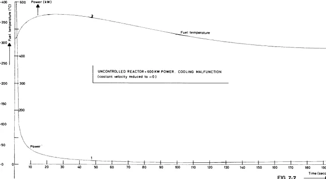
-7. Malfunctions

Control rod malfunctions occurring in the uncontrolled reac­ tor have been simulated as a part of reactor safety studies. The set of equations (2-4) was used for this purpose. We in­ vestigated the malfunctions of:

- the fast control rod (by inserting 10 pcm at 20 pcm/s) - the slow control rod (by inserting 40 pcm at O.83 pcm/s) - the regulation rod (by inserting 300 pcm at 3 pcm/s).

Now, in order to have a first assessment of the importance of a reduction in the values of the reactivity feedback coeffi­ cients, each malfunction was repeated changing these coeffi­ cients. Four cases were considered:

Case 1 Case 2

Case 3 Case 4

af

Reference value (-0.42pcm/^C) Half reference value

(-0.21pcm/°C) Reference.value (-0.42pcm/°C)

0

— — — — — — — — — — — — — — — — — — — — —

ag

Reference value (-0.80pcm/°C) Half reference value

(0.40pcm/°C) 0

Reference value (-0.80pcm/°C)

Ci

mml ï'

ΖΓ^ΤΊ; Γ:- '·ΐ:

CT

O-J

pc m/si..

r—400

—350 ï

n—600 Power (kW)

-300,

—250

— 200

—150

-100

-50

"— 0 0

î

--400

300

— 200

„ Power '

J L

Fuel temperature

UNCONTROLLED REACTOR = 600 KW POWER. COOLING MALFUNCTION (coolant velocity reduced to ~ 0 )

1 1 b I I

_ι

_ι

_ι

10 20 30 40 50 60 70 80 90 100 110 120 130 KO 150 160 170 180 190 200

FIG 7-7

Time (seconds)

►

72

-Conclusion

As may be noted, this study has been performed using exten­ sively only two programmes: the SAHYB-programme for simulation and the subroutine POLRT for finding the roots of polynominals. This meth od has proved to be powerful since it permitted

-in a short time and without any difficulty - to answer most questions about the SORA dynamics and control, such as: reac­ tor response to perturbations, start-up procedure, design of the fast control system, malfunctions, etc. Therefore, the initial choice of a digital computer for such a study seems retrospectively to be a good one.

Of interest also is the possibility of extending the simulation to the whole plant: the set of equations (6-4) may be completed with a'heat exchanger description and safety circuits. In this manner, a complete logical start-up procedure should be defined, However, the obtained results lie on the assumption of mean

73

Appendix 1 - Derivation of numerical values

for

a

steady-state condition at power

Let us assume a pulsed steady state condition at power P~ .

We may neglect the contribution of the source-term S ; then

we get the following set of equations for kinetics:

4140 c

K = 0,229 + 8,80 e

+ 0,0176 e = 1

*o = V

f

ΐ

ί

o> with Κ = 1

dC.

- # = ^ i

o -

i

io = °

w

Ρ = -2

from which

we

derive

w

= C

P

and successively;

β

1

-C

10 =

X 7

o

Η

-C

20

" A J

o

etc.

C

60

"XJ

o

for the set of equations "thermal description", we get:

0 = pP" - h-, (f

~ - f

)

r

o

Fs

fo

go

0

-

Fs <*fo - V

- - f c

V

c,in>

1 ι ° C

1 +

2vcT

74 ­

Τ are calculated successively. Results are given here below;

co J °

Ü

10 =

^ 7

F

o

C2 0 = ν 2 CF Po

C

30 " ν ­­J.

F

o

λ

3

C

40

^

F

o

C

50 =

"Tf

F

o

C6 0

= v

T

fo

c , i n

' V E " "

KT

3VT>

' Fs se c

pp" Lh

Τ ­ Τ + ° (1 + s c )

'go ­ ' e i n + hs c Π + 2VCc J

Tc,out,o = Tc,in + p Po "SVC~

c

Tco = Tc , m + 'Po

2ΎΟ-c