Munich Personal RePEc Archive
Expectations-Based
Reference-Dependent Preferences and
Asset Pricing
Pagel, Michaela
University of California at Berkeley
December 2012
Online at
https://mpra.ub.uni-muenchen.de/47933/
Expectations-based Reference-dependent Preferences
and Asset Pricing
Michaela Pagel
∗Department of Economics
University of California at Berkeley
December 28, 2012
Abstract
This paper incorporates expectations-based reference-dependent preferences into the canonical Lucas-tree asset-pricing economy. Expectations-based loss aver-sion increases the equity premium and decreases the consumption-wealth ratio, because uncertain fluctuations in consumption are perceived to be more painful. Moreover, because unexpected cuts in consumption are particularly painful, the agent wants to postpone such cuts to let his reference point decrease. Thus, even though shocks are i.i.d., loss aversion induces variation in the consumption-wealth ratio, which generates variation in the equity premium, expected returns, and pre-dictability. The level and variation in the equity premium and the predictability in returns match historical moments, but the associated variation in intertempo-ral substitution motives results in excessive variation in the risk-free rate. This effect can be partially offset with variation in expected consumption growth, het-eroskedasticity in consumption growth, or time-variant disaster risk. As a key contribution, I show that the preferences resolve the equity-premium puzzle and simultaneously imply plausible risk attitudes towards small and large wealth bets.
∗
E-mail: [email protected]. I am indebted to Adam Szeidl and Matthew Rabin for their extensive advice and support. I thank Martin Lettau, Nick Barberis, and Botond Koszegi, as well as my orals committee members Stefano DellaVigna and Ulrike Malmendier, Josh Schwartzstein, Ted O’Donoghue, David Laibson, and seminar participants at UC Berkeley, Yale, and the Olin Business School for their helpful comments and suggestions. All errors remain my own.
1
Introduction
Several leading asset-pricing models assume reference-dependent preferences that eval-uate consumption relative to a reference point. Campbell and Cochrane (1999) assume habit-formation1
preferences, and Benartzi and Thaler (1995), Barberis, Huang, and Santos (2001), and Yogo (2008) use prospect-theory2
preferences. Each of these models assume that the reference point is backward-looking and formalize it in specific ways. Moreover, the prospect-theory models specify utility directly over financial wealth in-stead of consumption, which implies a narrow-framing3
assumption. Koszegi and Rabin (2006, 2007, 2009) develop a new, generally-applicable model of reference-dependent preferences in a series of influential theory papers, which successfully explains an array of behavioral and experimental evidence. The preferences are based on consumption and offer a fully-endogenized reference-point specification, thereby eliminating one of the major degrees of freedom associated with prospect theory.
In an otherwise standard Lucas-tree model, expectations-based loss aversion intu-itively implies a first-order shift and variation in the consumption-wealth ratio; the latter of which is a new and distinct prediction in the prospect-theory asset-pricing literature. As a result, the model matches historical levels of the equity premium, its volatility, and the degree of predictability in returns. Remarkably, these implications are independent of common assumptions in the literature, such as a separate process for dividends or narrow framing.4
Moreover, I show that the preferences imply plausible risk attitudes towards small, medium, and large wealth bets and thus make a first step in explaining microeconomic evidence and resolving the equity-premium puzzle; this can be seen as a key contribution to the existing literature.
Expectations-based reference-dependent preferences consist of two components. “Con-sumption utility” is determined by con“Con-sumption and corresponds to the standard model of utility. Contemporaneous and prospective “gain-loss utility” is determined by a com-parison of current and future consumption with the reference point and corresponds to the prospect-theory model of utility. The latter component incorporates loss aversion; small losses are more painful than equal-sized gains are pleasurable. The reference point is stochastic and corresponds to the agent’s fully probabilistic rational beliefs about current and future consumption formed in the previous period. Then, the agent
1
Habit formation (Abel (1990)) is a preference theory saying that people’s utility function depends on the change in consumption rather than the level of consumption.
2
Prospect theory (Kahneman and Tversky (1979)) is a behavioral theory aimed to describe risk preferences elicited in experiments. The theory says that people care about gains and losses relative to a reference point, whereby small losses hurt more than equal-sized gains give pleasure, i.e., people are loss averse.
3
Narrow framing refers to the phenomenon that people appear to evaluate an offered gamble in isolation, rather than mixing it with existing risk or considering its actual implications for consumption instead of financial wealth.
4
A separate dividend process is typically assumed to reduce the contemporaneous correlation of consumption and returns; this, however, is not necessary in the basic model, which matches the contemporaneous correlation reasonably well.
compares consumption utility for each possible outcome under his updated beliefs with consumption utility for each possible outcome under his prior beliefs, and he experi-ences a corresponding sensation of gain or loss. Accordingly, the agent derives gain-loss utility from unexpected changes in present consumption and revisions in expectations over future consumption; therefore, gain-loss utility can be interpreted as utility over good and bad news.
This paper incorporates such “news-utility” preferences into an otherwise standard consumption-based asset-pricing model and solves for the rational-expectations equi-librium in closed form. The model environment is a simple endowment economy with log-normal consumption growth in the spirit of Lucas (1979). The Mehra and Prescott (1985) model – which shows that constant relative risk aversion preferences are incon-sistent with basic financial market moments – is preserved as a special case.
As a stepping stone to describing the model’s asset-pricing implications, I first ex-plain two predictions about the model’s consumption-wealth ratio.5
First, the consumption-wealth ratio is shifted down relative to the standard model. Because the agent is loss averse, he anticipates uncertain fluctuations in gain-loss utility that are painful on average. But, these fluctuations are less painful on a less steep part of the util-ity curve, which introduces an additional precautionary-savings motive. Second, the consumption-wealth ratio varies, in contrast to the standard model and despite the i.i.d. environment. Because the agent is loss averse relative to his expectations, he finds unexpected reductions in consumption more painful than expected reductions in consumption; hence, the agent wants to postpone unexpected reductions in con-sumption until his expectations will have decreased. More precisely, reducing future consumption automatically decreases the future reference point, whereas the present reference point is fixed. Consequently, reductions in future consumption are relatively less painful than reductions in present consumption. Finally, these two effects on the consumption-wealth ratio are first order as they depend on loss aversion.
These findings drive the model’s asset-pricing predictions. First, the shift of the consumption-wealth ratio is reflected in an increased mean equity premium. Because the agent is loss averse, he requires a high compensation for the painful fluctuations in consumption associated with uncertainty. Second, the variation in the consumption-wealth ratio is reflected in variation of expected returns. In bad times, the agent desires to consume more and save less. In general equilibrium, this desire increases the consumption-wealth ratio, decreases the price-consumption ratio, and thus increases expected returns. Accordingly, the model generates predictability: In bad times, a high consumption-wealth ratio predicts high future returns. Because high expected returns have high standard deviations, which increase the price of risk, expected excess returns are higher too. Thus, excess returns are predictable too.
I calibrate the news-utility preference parameters in line with microeconomic evi-dence and show that this calibration generates realistic attitudes towards small, medium,
5
and large wealth bets. Moreover, this calibration obtains a log equity premium of ap-proximately six percent with a standard deviation of nineteen percent and thus matches historical stock market data, even though consumption equals dividends in the basic Lucas-tree model.6
Moreover, I find variation in the consumption-wealth ratio around three percent and R2s in the predictability regressions of approximately ten percent. These values match the empirical findings of Lettau and Ludvigson (2001), who doc-ument the medium-term predictability properties of the consumption-wealth ratio.7
Besides, I show that such strong predictability of the consumption-wealth ratio on the return and excess return on the aggregate consumption claim is not generated by other leading asset-pricing models.
A misprediction of the model is strong variation in the risk-free rate, which is com-monly predicted by habit-formation models but not borne out by the data. In the event of adverse shock realizations, the agent dislikes immediate reductions in consumption and is unwilling to substitute intertemporally, which increases both the expected risky and risk-free rate of return. Although not reflected in aggregate data, this underlying time-variation in substitution motives may not be implausible in practice. Indeed, be-cause people are unwilling to substitute intertemporally in sometimes, they use credit cards and payday loans, thus borrowing at high interest rates. The intent of this paper is not to change the evidence-based utility function; rather, I take the variation in sub-stitution motives seriously and explore three model-environment extensions that partly offset the strong intertemporal substitution effects on the risk-free rate.
First, I assume variation in expected consumption growth, as in Bansal and Yaron (2004). Second, I assume variation in consumption growth volatility, i.e., heteroskedas-ticity in the consumption process, as in Campbell and Cochrane (1999). Third, I add disaster risk to the consumption process, so that there is a small probability that the agent suffers a large loss in consumption, as in Barro (2006, 2009). I find that news-utility preferences amplify disaster risk, because they feature “left-skewness aversion”, as opposed to standard prospect-theory preferences. The addition of heteroskedasticity or disaster risk introduces variation in the strength of the precautionary savings motive, which partly offsets the effects of the variation in substitution motives on the risk-free rate, adds variation in the price of risk, and generates long-horizon predictability.
Last, I quickly describe the model’s welfare implications. News utility increases the costs of business cycle fluctuations, in the spirit of Lucas (1978), to realistic levels.
6
The model’s equity premium and its volatility are increasing in the model’s simulation frequency, which, therefore, constitutes a major calibrational degree of freedom. Taking the calibration as given, I choose a one-and-a-half month frequency that happens to match both the historical equity premium and its volatility. The model’s frequency matters due to the famous idea of myopic loss aversion (Benartzi and Thaler (1995)): In contrast to standard preferences, loss aversion implies that a cumulative lottery becomes inherently less attractive when its independent draws are evaluated more rather than less frequently. I am intrigued by the idea that people require a large compensation for risk, because they are subject to painful fluctuations in beliefs when they worry frequently about small fluctuations in their future consumption.
7
Moreover, the first welfare theorem does not hold, because the preferences are subject to a beliefs-based time inconsistency.8
After a literature review, I present the preferences, the model environment, and the Markovian rational-expectations equilibrium in sections 3.1 and 3.2. Then, in section 3.3, I explain the model’s predictions about the consumption-wealth ratio. In section 4.1, I discuss the model’s asset-pricing implications and calibrate the model to gauge its quantitative implications in section 4.2. In section 5, I extend the model to allow for time-variant expected consumption growth, time-variant volatility, and disaster risk. Section 6 explains the model’s implications for welfare. Finally, section 7 concludes.
2
Comparison to the literature
In recent years, loss aversion became a widely accepted explanation for the equity-premium puzzle. I further this literature by showing that most results carry over to a new, micro-founded preference specification, which has been used in a variety of con-texts to explain behavioral and experimental evidence.9
As a result, major degrees of freedom associated with prospect theory can be eliminated: The reference point is fully endogenous, and tight ranges exist for all preference parameters. However, a different calibrational degree of freedom emerges, which did not receive much attention in static applications; the length of each time period, or the model’s simulation frequency. Sim-ulating the model at higher frequency increases the equity premium, because the loss averse agent finds many independent draws of a gamble less attractive than all these
8
Lacking an appropriate commitment device, the agent optimizes in each period, taking his beliefs as given. Thus, he is inclined to positively surprise himself with extra consumption in each period. Consequently, the agent is forced to choose a sub-optimal consumption path, which differs from the expected-utility-maximizing path on which the agent jointly optimizes over consumption and beliefs.
9
gambles’ cumulative outcome.10
I calibrate the model in line with microeconomic evi-dence and then choose a one-and-a-half month frequency that matches both the equity premium and its volatility, i.e., the historical risk-return trade off. Moreover, I show that the preferences are tractable in a multi-period, continuous-outcome framework; this is not readily apparent given their high level of complexity.
While other models are equally able to match asset-pricing moments, news util-ity simultaneously explains behavior observed in microeconomic studies. I show that the preference parameters induce realistic attitudes towards small, medium, and large wealth bets, which are not well explained by other preference specifications.11
There-fore, I take a step forward in developing a framework that can match both macroe-conomic and microemacroe-conomic behavior. This improved micro foundation has desirable implications, namely variation in the consumption-wealth ratio, expected returns, and predictability, which matches the evidence provided by Lettau and Ludvigson (2001) better than those of the standard, habit-formation, or long-run risk models. But, the well-known problem that the risk-free rate responds strongly to intertemporal smooth-ing incentives is not resolved. Time-variant consumption growth, heteroskedasticity, or disaster risk is needed to offset some of the effects on the risk-free rate.
The pioneering prospect-theory asset-pricing papers, Barberis, Huang, and Santos (2001) and Benartzi and Thaler (1995), specify gain-loss utility directly over fluctua-tions in financial wealth. In so doing, the authors make an assumption about narrow framing. The agent narrowly frames the stock market, because he experiences gain-loss utility directly over financial wealth. In contrast, the news-utility agent experi-ences gain-loss utility over the implications of his financial wealth for contemporaneous and future consumption. The news-utility model yields a high equity premium with-out narrow framing, because the agent experiences gain-loss utility over fluctuations in contemporaneous consumption and the entire stream of future consumption, which makes uncertainty sufficiently painful. Yogo (2008) argues also that fluctuations in con-sumption rather than financial wealth are the relevant measure of risk. The author’s preferences are a mixture of habit formation and prospect theory and yield a high eq-uity premium; variation in the risk-free rate is mitigated via persistence in the habit process. The main difference with respect to Koszegi and Rabin (2009) preferences is that the reference point is backward-looking. In contrast, Andries (2011) incorporates loss aversion into a consumption-based asset pricing model and explains positive skew-ness premia and a flat security market line. The agent’s value function features a kink at the expected value of consumption, which nicely captures forward-looking reference
10
This result relates to myopic loss aversion and the Samuelson’s colleague story (Benartzi and Thaler (1995)).
11
dependence. However, because the agent exhibits reference-dependent preferences with respect to his future value rather than present consumption, the underlying preference mechanisms and predictions are very different from those I obtain.
Campbell and Cochrane (1999) show that habit formation matches a range of asset-pricing moments. Moreover, this paper’s main prediction, the variation in the agent’s willingness to substitute intertemporally, has also been emphasized by Campbell and Cochrane (1999). But, the authors exactly offset this variation in intertemporal substi-tution motives by a habit process that features variation in the agent’s precautionary-savings motive. Furthermore, because the agent’s habit increases the curvature of the value function, the agent’s effective risk aversion is quite high and becomes the main variability-driving mechanism. The same holds true for Barberis, Huang, and Santos (2001), variation in the coefficient of loss aversion introduces predictability, whereas the additively separable gain-loss components over financial wealth yields a constant consumption-wealth ratio and risk-free rate. In the news-utility model, effective risk aversion is constant and equals the coefficient of relative risk aversion. The model retains the power utility property that the curvature of the value function is solely de-termined by the coefficient of relative risk aversion, as gain-loss utility is proportional to consumption utility.
Routledge and Zin (2010) assume generalized disappointment-aversion preferences and show that these are consistent with basic financial market moments. The model has been extended to long-run risk by Bonomo, Garcia, Meddahi, and Tedongap (2011). However, these models rely on high risk aversion in low states of the world when the agent is likely to be disappointed, as habit-formation preferences do.12
Furthermore, Campanale, Castro, and Clementi (2010) assume disappointment-aversion preferences in a production economy. In this model the excessive volatility of the risk-free rate can be reduced by assuming a high intertemporal elasticity of substitution. However, the variation in returns is acyclical by construction, which rules out predictability.13
This paper contributes to the literature by incorporating a preference specification, which has proven to be consistent with an array of micro evidence in a variety of domains. Thus, I can relate microeconomic evidence to the model’s asset-pricing im-plications and the intuition of which, pin down narrow ranges for all parameters, and simultaneously match risk attitudes over small, medium, and large stakes.
12
Strong variation in effective risk aversion has problems to robustly match evidence on risk attitudes towards wealth bets and is contradicted by portfolio-choice data (Brunnermeier and Nagel (2008)).
13
3
The Model
3.1
Expectations-based reference-dependent preferences
I assume expectations-based reference-dependent preferences, as specified in Koszegi and Rabin (2009). Instantaneous utility in each period is the sum of consumption utility and loss utility. The latter component consists of “contemporaneous” gain-loss utility about current consumption and “prospective” gain-gain-loss utility about the entire stream of future consumption. Thus, total instantaneous utility in period t is given by
Ut=u(Ct) +n(Ct, FCt−t1) +γ ∞
X
τ=1
βτn(Ft,t−1
Ct+τ). (1)
The first term in equation (1) corresponds to consumption utility in period t, which is a power-utility function u(c) = c1−θ
1−θ. The following terms are defined over both consumption and the agent’s “beliefs” about consumption, which I explicitly define below. Throughout the paper, I assume rational expectations such that the agent’s beliefs about any of the model’s variables equal the objective probabilities determined by the economic environment.
Definition 1. Let It denote the agent’s information set in some period t ≤ t +τ, then the agent’s probabilistic beliefs about consumption in periodt+τ, conditional on periodt information, is denoted byFCtt+τ(c) =P r(Ct+τ < c|It)andF
t+τ
Ct+τ is degenerate.
To understand the following terms in equation (1), first note that the reference point in period t are the fully probabilistic beliefs about consumption in periodt and all future periods t+τ, given the information available in period t−1. According to definition 1, the agent’s beliefs formed in periodt−1 about period t+τ consumption are denoted byFt−1
Ct+τ. Thus, the second term in equation (1),n(Ct, F
t−1
Ct ), corresponds
to gain-loss utility in periodt over contemporaneous consumption. Gain-loss utility is determined by a piecewise linear value functionµ(·)with slopeηand a coefficient of loss aversion λ, i.e., µ(x) = ηx for x > 0 and µ(x) = ηλx for x ≤0. The parameter η > 0
weights the gain-loss utility component relative to the consumption utility component and λ > 1 implies that losses are weighed more heavily than gains; the agent is loss averse. Because the agent compares his actual contemporaneous consumption with his prior beliefs, he experiences gain-loss utility over “news” about contemporaneous consumption as follows
n(Ct, Ftt−1(C t−1 t )) =
ˆ ∞
0
µ(u(Ct)−u(c))dFCt−t1(c)
=η ˆ Ct
0
(u(Ct)−u(c))dFCt−t1(c) +ηλ
ˆ ∞
Ct
(u(Ct)−u(c))dFCt−t1(c). (2)
The third term in equation (1), γP∞
τ=1βτn(F t,t−1
Ct+τ), corresponds to prospective
gain-loss utility in period t over the entire stream of future consumption. Prospective gain-loss utility about period t+τ consumption, n(Ft,t−1
Ct+τ), depends on F
t−1
beliefs with which he entered the period, and on FCtt+τ, the agent’s updated beliefs
about periodt+τ consumption. Ft−1
Ct+τ and F
t
Ct+τ are correlated distribution functions,
because future uncertainty is contained in both prior and updated beliefs about Ct+τ. Thus, there exists a joint distribution, which I denote byFt,t−1
Ct+τ 6=F
t Ct+τF
t−1
Ct+τ. Because
the agent compares his new beliefs with his prior beliefs, he experiences gain-loss utility over “news” about future consumption
n(Ft,t−1
Ct+τ) =
ˆ ∞
0 ˆ ∞
0
µ(u(c)−u(r))dFt,t−1
Ct+τ(c, r). (3)
Both contemporaneous and prospective gain-loss utility correspond to an outcome-wise comparison as assumed in Koszegi and Rabin (2006, 2007).14
Moreover, the agent discounts prospective gain-loss utility exponentially by β, the standard agent’s con-sumption utility discount factor; and prospective gain-loss utility is subject to another discount factor γ relative to contemporaneous gain-loss utility, so that the agent puts a weight γβτ <1 on prospective gain-loss utility about consumption in periodt+τ.
Because both contemporaneous and prospective gain-loss utility are experienced over news, the preferences are referred to as “news utility”.
3.2
The model environment and equilibrium
The model environment. I consider a Lucas (1979) tree model in which the sole source of consumption is an everlasting tree that produces Ct units of consumption each period t. I assume that consumption growth is log-normal, following Mehra and Prescott (1985). Thus, the endowment economy’s exogenous consumption process is given by
log(Ct+1
Ct
) = µc +εt+1 with εt+1 ∼N(0, σc2). (4) The price of the Lucas tree in each period t is Pt. Moreover, there exists a risk-free asset in zero net supply with returnRft+1. The periodt+ 1 return of holding the Lucas tree is then Rt+1 = Pt+1P+Ct t+1. Each period t, the agent faces the price of the Lucas treePt and the risk-free returnRft+1 and, acting as a price taker, optimally decides how much to consumeC∗
t and how much to invest in the risky asset α∗t. 15
14
The outcome-wise comparison of Koszegi and Rabin (2006, 2007) has been generalized to an ordered comparison in Koszegi and Rabin (2009), because the agent would otherwise experience gain-loss disutility over future uncertainty even if no update in information takes place. I circumvent this problem by explicitly noting that prior and new beliefs about consumption are correlated, i.e., I generalize the gain-loss formula of Koszegi and Rabin (2006, 2007)
n(Fc, Fr) =
ˆ ∞
0
ˆ ∞
0
µ(u(c)−u(r))dFr(r)dFc(c) to n(Fc,r) =
ˆ ∞
0
ˆ ∞
0
µ(u(c)−u(r))dFc,r(c, r).
The ordered comparison yields qualitatively and quantitatively similar results but the model’s solution is not as tractable.
15
consump-Equilibrium prices and definition. Because the agent fully updates his beliefs each period and the consumption process is i.i.d., I look for an equilibrium price and risk-free return process that is “Markovian” in the sense that the price-consumption ratio depends on the current shock only.
Definition 2. The price process {Pt}∞t=0 and risk-free return process {Rft+1}∞t=0 are Markovian if, in each period t, the price-consumption ratio Pt
Ct and the risk-free return
Rft+1 depend on the realization of the shock εt only, such that PCtt =p(εt) and Rft+1 =
r(εt)with the functionsp(·)andr(·)being independent of calender timetor endowment Ct.
Facing Markovian prices and returns, the agent’s maximization problem in periodt
is given by
maxCt{u(Ct) +n(Ct, F
t−1
Ct ) +γ ∞
X
τ=1
βτn(Ft,t−1
Ct+τ) +Et[ ∞
X
τ=1
βτUt+τ]}. (5)
The agent’s wealth in the beginning of period t, Wt, is determined by the portfolio return Rpt, which depends on the risky return realization Rt, the risk-free return Rft, and previous period’s optimal portfolio shareαt−1. The budget constraint is
Wt= (Wt−1−Ct−1)Rpt = (Wt−1−Ct−1)(Rft +αt−1(Rt−Rft)). (6) In each period t, the agent optimally decides how much to consume C∗
t, how much to investWt−Ct∗, and how much to invest in the risky assetα∗t. In equilibrium, the price of the treePt=Wt−Ct adjusts so that the single agent in the model always chooses to hold the entire tree, i.e.,α∗
t = 1 for all t, and consume the tree’s entire payoff Ct∗ =Ct for alltas determined by the endowment economy’s exogenous consumption process (4). In the following, I derive the “Markovian rational-expectations equilibrium” recursively; in the Lucas-tree model, it corresponds to the preferred-personal equilibrium, as defined in Koszegi and Rabin (2006).16
Definition 3. The Markovian rational-expectations equilibrium consists of a Marko-vian price process {Pt = Ctp(εt)}∞t=0 and a risk-free return process {R
f
t+1 = r(εt)}∞t=0 such that the solution {C∗
t, α∗t}∞t=0 of the price-taker’s maximization problem (5) sub-ject to the budget constraint (6) satisfies goods market clearing{C∗
t =Ct}∞t=0 and asset market clearing{α∗
t = 1}∞t=0.
tion process, i.e.,Ft
Ct+τ(c) =P r(Ct+τ < c|It),It={Ct, Pt, εt}, and
Ct+1
Ct =e
µc+εt+1 ∼log−N(µ
c, σc2)
for anyt∈[0,∞)such thatFt
Ct+τ =log−N(log(Ct) +τ µc, τ 2σ2
c)for anyτ >0.
16
Equilibrium existence and structure.
Proposition 1. A Markovian rational-expectations equilibrium exists.
This and the following propositions’ proofs can be found in appendices B.1 to E.1. The equilibrium has a very simple structure and can be derived in closed form. In each period t, optimal consumption C∗
t is a fraction of current wealth Wt such that C∗
t =Wtρt. As appendix B.2 shows, the consumption-wealth ratio ρt is ρt=
C∗
t Wt
= 1
1 + Q+Ω+γQΩ+γQ(ηF(εt)+ηλ(1−F(εt)))
1+ηF(εt)+ηλ(1−F(εt))
. (7)
Here, F(·) denotes the cumulative normal distribution function N(0, σc) and Q and Ω are determined by exogenous parameters. Thus, ρt varies with the realization of εt, is i.i.d., independent of calender timet, or current endowmentCt. The price-consumption ratio is Pt
Ct =
1−ρt
ρt . The agent’s value function is proportional to the power utility of
wealth Vt = u(Wt)Ψt. Ψt varies with the realization of εt, is i.i.d., independent of calendar time t, or current endowmentCt. I now explain the news-utility agent’s first-order condition in detail to build intuition for Qand Ωand to clarify why and how ρt varies with εt.
3.3
Predictions about the consumption-wealth ratio
Before turning to the model’s asset pricing implications, I describe the agent’s first-order condition to provide intuition for two predictions about the agent’s consumption-wealth ratio, which are formalized in propositions 2 and 3 and illustrated in figure 1. Although the first-order condition appears complicated, the terms can be easily understood one component at a time. The agent’s consumption-wealth ratioρt, equation 7, results from the model’s first-order condition
C−θ
t (1 +ηF(εt) +ηλ(1−F(εt)
| {z }
contemporaneous gain-loss
)
= ( ρt 1−ρt
)1−θ(W
t−Ct)−θ(Q+ Ω +γΩQ
| {z }
=−dβEt[u(WtdCt+1)Ψt+1]
+γQ(ηF(εt) +ηλ(1−F(εt))
| {z }
prospective gain-loss
)). (8)
First, for η = 0, the model collapses to the standard consumption-based asset-pricing model with constant relative risk aversion and log-normal consumption growth assumed by Mehra and Prescott (1985) among many others. The first-order condition becomes
C−θ t = (
ρs
1−ρs) 1−θ
The shift in the consumption-wealth ratio. The left hand side of the first-order condition, equation (8), is simply determined by marginal consumption and gain-loss utility over contemporaneous consumption. Marginal gain-loss utility is given by the states that would have promised less consumption Ft−1
Ct (Ct), weighted by η, or more
consumption1−Ft−1
Ct (Ct), weighted byηλ, i.e.,
∂n(Ct,Ft −1
Ct )
∂Ct =u ′(C
t)(ηFCt−t1(Ct) +ηλ(1−
Ft−1
Ct (Ct))). A key technical insight here allows me to simplify the marginal gain-loss
utility term: In the Lucas-tree model, equilibrium consumption is determined by the realization of the shockεt, which allows me to simplifyFCt−t1(Ct) =F(εt).
Let me turn to the right hand side of equation (8). The first term represents the marginal value of savings−dβEt[u(Wt+1)Ψt+1]
dCt = u ′(W
t−Ct)(Q+ Ω +γΩQ) with Q and
Ωdetermined by exogenous parameters. In the standard model, the marginal value of savings is given byu′(W
t−Ct)Q. Thus, Q represents the discounted stream of future consumption utility, and Ω represents expected gain-loss utility; the marginal value of savings is determined by Q+ Ω +γΩQ, the sum of expected consumption utility, expected contemporaneous gain-loss utility, and expected prospective gain-loss utility discounted by γ. Accordingly, if expected gain-loss disutility is positive Ω > 0, then the marginal value of saving increases relative to the standard model. The underlying intuition is that the agent anticipates gain-loss disutility that is proportional to marginal consumption utility. Thus, fluctuations are less painful on a less steep part of the utility curve, and the agent has an additional incentive to increase savings. Moreover, it can be shown that the additional precautionary-savings motive is first-order, i.e., ∂Ω
∂σc|σc=0 >0,
because it depends on concavity of the utility curve rather than prudence as in the standard model.
However, if the agent discounts news about the future γ < 1 he has an additional reason to consume more today, because positive news about contemporaneous con-sumption are overweighted. Thus, the additional precautionary-savings motive results in the consumption-wealth ratio being lower than in the standard model, if the agent does not discount future news too highlyγ > γ¯. These ideas can be formalized in the following proposition.
Proposition 2. If θ > 1 and γ > γ¯ with ¯γ = ηλ−
Ω
Q
Ω+ηλ < 1 then, for all realizations of εt, the consumption-wealth ratio in the news-utility model is lower than in the standard
model ρt< ρs. Moreover, γ¯ is decreasing in the news-utility parameters ∂λ∂¯γ,∂¯∂ηγ ≤0. 17
Koszegi and Rabin (2009) state in proposition 8 that news-utility introduces an additional first-order precautionary savings motive in a two-period two-outcome model. Proposition 8 carries over only for θ > 1, because I consider multiplicative instead of additive shocks. Multiplicative shocks imply that savings increase the absolute value of tomorrow’s wealth bet, which the news-utility agent dislikes. For θ < 1, this effect dominates the intertemporal smoothing desire. For log utility θ = 1, the two motives
17
Ifθ >0and η−ΩQ
Ω+η < γ <γ¯ thenρsandρtcross atεt= ¯εtandεt¯ is decreasing in the news-utility
parameters ∂ε¯t
∂λ, ∂¯εt
exactly offset each other andΩ = 0. Thus, if θ = 1 and γ = 1, the news-utility model becomes observationally equivalent to the standard model.18
Variation in the consumption-wealth ratio. Let me move on to the second part on the right hand side in the first-order condition (8) that represents marginal prospec-tive gain-loss utility. In the absence of expected gain-loss disutilityΩ = 0 and prospec-tive gain-loss discounting γ = 1, marginal contemporaneous and prospective gain-loss utilities would cancel out. Then, I would be back in the standard model with a propor-tional response of consumption to wealth. However, contemporaneous marginal utility is driven above future marginal utility due to the additional marginal value of savings
Ω>0 so thatQ+ Ω +γQΩ6=γQ. Thus, the consumption-wealth ratio ρt varies with the realization of εt.
Moreover, the consumption-wealth ratio is decreasing forθ >1. Because unexpected losses are particularly painful, the agent consumes relatively more of his wealth in the event of an adverse shock. I first outline a simplified intuition: If the agent encounters an adverse shock, decreasing consumption below expectations today is more painful than decreasing consumption tomorrow when the reference point will have decreased. If the agent encounters a positive shock he experiences less painful gain-loss fluctuations today relative to tomorrow when the reference point will have increased. Thus, the agent wants to delay the consumption response to shocks, which makes the consumption-wealth ratio variable. More formally, in the event of an adverse shock, present marginal gain-loss utility is high relative to future marginal gain-loss utility. Today’s reference point is invariable, whereas tomorrow’s reference point will have adjusted to today’s shock. Thus, future marginal gain-loss utility is constant whereas present marginal gain-loss is high, and the agent wants to consume relatively more today and relatively less tomorrow.19
The following proposition formalizes this idea.
Proposition 3. If θ 6= 1 news utility introduces variation in the consumption-wealth ratio ∂ρt
∂εt 6= 0. Moreover, for θ > 1 the consumption-wealth ratio is decreasing
∂ρt
∂εt <0.
The model’s implications are illustrated in figure 1, which displays the consumption-wealth ratioρt as a function of the shock to consumption growth and contrasts it with the standard agent’s ratio for two levels if σc. The corresponding calibration is given in table 3 with λ = 2. News-utility preferences predict a downward shift and specific variation in the consumption-wealth ratio. The shape is driven by marginal gain-loss utility, which depends on the shock distribution ηF(εt) +ηλ(1−F(εt)) ∈ [η, ηλ]. As εt is characterized by a bell-shaped distribution, the variation in the consumption-wealth ratio is bounded. The agent experiences gain-loss utility over all other states he might have been in weighted by their probabilities. For extreme realizations of
18
This result is analogous to a result for quasi-hyperbolic discounting obtained by Barro (1999).
19
εt, the consumption-wealth ratio approaches its limits because the states near these realizations have very low probabilities. ρt and ρs are displayed for two levels of σc, which illustrates that, for a small increase in σc, the downward shift in ρt is larger than the downward shift inρs, because the additional precautionary savings motive is a first-order effect, i.e., ∂ρt
∂σc|σc→0 >0, while the standard precautionary-savings motive
[image:15.612.152.455.195.437.2]is second order.
Figure 1: Consumption-wealth ratio ρt in the news-utility and standard models.
Furthermore, the steepness or responsiveness of the consumption-wealth ratio near the center of the distribution depends on the amount of economic uncertaintyσc. The responsiveness of the consumption-wealth ratio is determined by the extent of pain or pleasure induced by gain-loss utility that is generally reduced for wider prior distri-butions. For example, a moderately bad realization feels less painful if the previously expected distribution was relatively less narrow; accordingly, the agent does not feel the need to respond as much. Finally, the consumption-wealth ratio is skewed in the sense that the agent underconsumes more in good times than he overconsumes in bad times. Adverse shocks are over-weighted and thus more effectively alleviated by previ-ously expected uncertainty. Accordingly, the consumption-wealth ratio becomes more skewed when uncertainty increases.20
20
This asymmetry can be illustrated by an increase in economic volatility σc. The consumption-wealth ratio shifts down and becomes more skewed. In the event of an overall negative surprise,
4
Asset Pricing
Now I turn to the model’s asset-pricing implications. First, I derive the expected risky return, the risk-free return, and the equity premium. Then I illustrate the model’s main asset-pricing predictions, namely variation in expected returns, the equity premium, and predictability. I aim to build intuition for these asset-pricing results by connecting them back to my prior theoretical results about the consumption-wealth ratio. Proposition 4 formalizes the main idea. In turn, I calibrate the model to gauge its quantitative performance in section 4.2 and compare them with the asset-pricing literature.
4.1
Predictions about expected returns and the equity premium
Expected returns and the equity premium. The return of holding the entire Lucas tree is Rt+1 = Pt+1P+Ct t+1. I can rewrite the expected risky return in terms of the consumption-wealth ratioρt and consumption growth CCt+1
t by taking expectations and
noting thatPt=Wt−Ct=Ct1−ρtρt, i.e.,
Et[Rt+1] = ρt
1−ρt Et[
1
ρt+1 Ct+1
Ct
]. (10)
Et[ρt1+1CCt+1t ] is constant because consumption growth CCt+1t =eµc+εt+1 and next period’s consumption-wealth ratio ρt+1 are i.i.d., as reported in definition 2 such that PCtt+1+1 =
p(εt+1) = 1−ρtρ+1t+1. However, Et[Rt+1] varies with the consumption-wealth ratio ρt.
I can rewrite the first-order condition as 1 = Et[Mt+1Rt+1], which gives rise to the agent’s stochastic discount factor Mt+1 derived in appendix B.2. The risk-free return is the inverse of the conditional expectation of the stochastic discount factor
Rt+1f = 1
Et[Mt+1]
= ρt 1−ρt
(Q+ Ω +γΩQ)Et[β( Ct+1
Ct
1
ρt+1
)−θΨ
t+1]−1. (11) Et[β(CCt+1t ρt1+1)−θΨt+1]−1 is constant because consumption growth CCt+1t = eµc+εt+1, the next period’s consumption-wealth ratio ρt+1, and the value function’s proportionality factor Ψt+1 are i.i.d. However, Rft+1 varies with the consumption-wealth ratio ρt. The equity premium
Et[Rt+1]−Rft+1 = ρt
1−ρt
(Et[
1
ρt+1 Ct+1
Ct
]−(Q+Ω+γΩQ)Et[β( Ct+1
Ct
1
ρt+1
)−θΨ
t+1]−1) (12) is characterized by a constant price of risk. The price of risk and the conditional Sharpe ratioSt = Et[Rt+1−R
f t]
σt(Rt+1) are constant, because the agent holds the entire stock market and
thus faces the same risk each period. However, the quantity of riskσt(Rt+1)varies with the consumption-wealth ratioρt.
Variation in expected returns and predictability. I have shown that the ex-pected risky return, the risk-free return, and the equity premium vary with the consumption-wealth ratio ρt. The news-utility implications about the location and shape of the consumption-wealth ratio ρt, which are formalized in propositions 2 and 3, directly carry over to the expected return, the risk-free return, and the equity premium. The variation in the expected risky return is generated by the general-equilibrium nature of the model and driven by variation in the agent’s willingness to substitute intertempo-rally as reflected by variation inρt.
In bad states of the world the agent would like to delay adjustments in consumption to let his reference point adjust. To induce the agent to consume his endowment, the price of the Lucas tree must be low and expected returns have to be high. Thus, despite the i.i.d. environment, the expected risky return varies to make the agent willing to hold the entire tree each period. Moreover, the variation in the consumption-wealth ratio generates return predictability. In particular, the realization of εt predicts the one-period ahead returnRt+1. Ifεt is low then ρtthe consumption-wealth ratio is high and the one-period ahead return is high; hence, the consumption-wealth ratio positively predicts one-period ahead returns. Moreover, this mechanism generates predictability in excess returns through the consumption-wealth ratio. Bad states predict high fu-ture returns, and this implies that the standard deviation of returns is also high and the expected equity premium varies with εt. Using the same argument as above, the realization ofεt then predicts the one-period ahead excess return Rt+1−Rft+1.
The following proposition formalizes the model’s implications for variation and pre-dictability in returns and the equity premium.
Proposition 4. If θ > 1 then the realization of the shock εt negatively impacts the
expected risky return ∂Et[Rt+1]
∂εt < 0, risk-free return
∂Rft
∂εt < 0, and equity premium
∂(Et[Rt+1]−Rft+1)
∂εt < 0. This implies predictive power of the period t consumption-wealth ratioρt regarding the period t+ 1 return Rt+1 and excess return Rt+1−Rt+1f .
For illustration, figure 2 in appendix A compares the annualized news-utility return and equity premium with the standard model’s ones under the calibration in table 3 with
λ = 2. The expected equity premium amounts to approximately ten percent for low values of εt and three percent for high values of εt. The high equity premium reflects that the news-utility agent perceives uncertain fluctuations in consumption as being much more painful than the standard agent. The equity premium’s variation stems from variation in the quantity of risk as a result of varying intertemporal smoothing incentives. But, the figure also illustrates how the model fails to predict reality: The risk-free return varies considerably, a phenomenon not observed in aggregate data.21
21
4.2
Basic model: Calibration and moments
In the following, I calibrate the model to gauge its quantitative performance. Before assessing the model’s ability to match asset-pricing moments, I illustrate the agent’s risk attitudes towards small and large wealth bets. I show that the news-utility model is able to simultaneously match evidence on small-scale and large-scale risk aversion.
4.2.1 Risk attitudes over small and large stakes.
Before moving on to the model’s asset-pricing moments I illustrate which news-utility parameter values, i.e., η, λ, and γ, are consistent with existing micro-evidence on risk preferences over small and large stakes and time preferences. I first show that the news-utility model does not generate high equity premia by secretly curving the value function to generate high effective risk aversion. On the contrary, the news-utility model retains a value function with constant curvature, because it is proportional to the power utility of wealth, i.e.,Vt=u(Wt)Ψt such that RRAt=−WtV
′′ t
V′ t =θ.
22
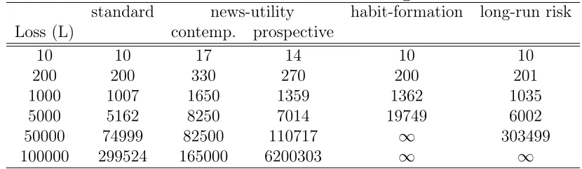
In table 1, I illustrate the risk preferences over gambles of various stakes of the standard, news-utility, habit-formation (Campbell and Cochrane (1999)), and long-run risk (Bansal and Yaron (2004)) agents. In particular, I analyze a range of 50-50 win G or lose L gambles at an initial wealth level of 300,000 in the spirit of Rabin (2001) and Chetty and Szeidl (2007). I elicit the agents’ risk attitudes by assuming that each of them is presented the gamble after the shock to periodtconsumption growth has been realized and all consumptionCtin periodthas taken place. Thus, the news-utility agent will experience merely prospective loss utility rather than contemporaneous gain-loss utility over the gamble’s outcome. In appendix B.6, I show that the news-utility agent is just indifferent to the gamble if
(Q+ Ω +γQΩ)u( ¯Wt) = γ(0.5η(u( ¯Wt+G)−u( ¯Wt))Q+ηλ0.5(u( ¯Wt−L)−u( ¯Wt))Q)
+ (Q+ Ω +γQΩ)(0.5u( ¯Wt+G) + 0.5u( ¯Wt−L)). (13) The first part on the right hand side of equation (13) represents prospective gain-loss utility, while the second part represents the same value comparison as done by the standard agent, i.e., u( ¯Wt) ≶ 0.5u( ¯Wt+G) + 0.5u( ¯Wt−L). Thus, if γ were zero the news-utility agent’s risk attitudes would be the exact same as the standard agent’s ones. Moreover, if L and G are small butG > L this second part will certainly be positive as
u(·) is almost linear, but the first part will induce prospect-theory risk preferences over future consumption. Although solelyλdetermines the sign of prospective gain-loss util-ity, there are restrictions on the other parameters, because the positivity of the second part may dominate the negativity of the first part if γ is small. Empirical estimates for the quasi-hyperbolic parameterβ in the βδ−model typically range between 0.7 and
22
0.8 (e.g., Laibson, Repetto, and Tobacman (forthcoming)). Thus, the experimental and field evidence on agent’s attitudes towards intertemporal consumption trade offs dictates a choice of γ ≈0.8 when β ≈1.
Simultaneously, the model should match risk attitudes towards bets about immedi-ate consumption, which are determined solely byηand λ, because it can be reasonably assumed that utility over immediate consumption is linear. Thus,η = 1 and λ≈2.5 is dictated by the laboratory evidence on loss aversion over immediate consumption, i.e., the endowment effect literature Kahneman, Knetsch, and Thaler (1990).23
In table 1, I calculate the required G for each value of L to make each agent just indifferent between accepting or rejecting a 50-50 win G or lose L gamble at wealth level
¯
Wt= 300,000. It can be seen that the news-utility agent’s risk attitudes take reasonable values for small, medium, and large stakes.24
In contrast, the standard and long-run risk agents are risk neutral for small stakes and almost risk neutral for medium stakes. The habit-formation agent is risk neutral for small stakes, reasonably risk averse for medium stakes, but that makes him unreasonably risk averse for large stakes. Campbell and Cochrane (1999) also discuss this finding and indicate that the curvature of the habit-formation agent’s value function is approximately 80 at the steady-state surplus-consumption ratio; thus, the habit-formation agent behaves similarly to a standard agent withθ = 80. The long-run risk agent behaves similarly to a standard agent with
θ = 10, the choice of Bansal and Yaron (2004). Moreover, it can be inferred from this discussion that the disappointment-aversion model (Routledge and Zin (2010)) does not
23
Let me take a concrete example from Kahneman, Knetsch, and Thaler (1990) assuming that utility over mugs, pens, and small amounts of money is linear. Kahneman, Knetsch, and Thaler (1990) hand out mugs to half the subjects and ask those who did not receive one about their willingness to pay and those who received one about their willingness to accept when selling the mug. The authors observe that the median willingness to pay for the mug is $2.75 whereas the willingness to accept is $5.25. Accordingly, I can infer(1 +η)u(mug) = (1 +ηλ)2.25and(1 +ηλ)u(mug) = (1 +η)5.25which implies that λ ≈ 3 when η ≈ 1. For the pen experiment I also obtain λ ≈3. Unfortunately, so far I can
only jointly identifyη and λ. If the news-utility agent exhibits only gain-loss utility I would obtain
ηλ2.25≈5.25andη2.25≈2.25, i.e.,λ≈2.3andη≈1both identified. Alternatively, if I assume that the market price for mugs (or pens), which is $6 in the experiment (or $3.75), equals(1 +η)u(mug)
(or (1 +η)u(pen)) I can estimateη = 0.74and λ = 2.03 for the mug experiment and η = 1.09and
λ= 2.1 for the pen experiment. These latter assumptions are reasonable given the induced-market experiments of Kahneman, Knetsch, and Thaler (1990). η = 1and λ ≈2.5 thus seem a reasonable choice and has been typically used in the literature for the static preferences.
24
Table 1: Risk attitudes over small and large wealth bets
standard news-utility habit-formation long-run risk Loss (L) contemp. prospective
10 10 17 14 10 10
200 200 330 270 200 201
1000 1007 1650 1359 1362 1035 5000 5162 8250 7014 19749 6002 50000 74999 82500 110717 ∞ 303499 100000 299524 165000 6200303 ∞ ∞
For each loss L the table’s entries show the required gain G to make each agent indifferent between accepting and rejecting a 50-50 gamble win G or lose L at wealth level 300,000.
robustly match risk attitudes towards small and large wealth bets, because the agent is not necessarily “at the kink”. The asset-pricing theories based on prospect theory (Barberis, Huang, and Santos (2001); Benartzi and Thaler (1995)) imply plausible attitudes towards small and large wealth bets but not consumption bets and are thus inconsistent with the endowment-effect evidence.
4.2.2 Calibration and asset-pricing moments
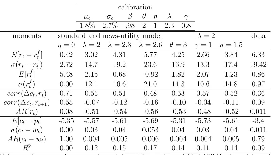
Calibration. Table 3 in appendix A displays the calibration and the resulting mo-ments of the news-utility and standard models, a short version of which is table 2. I begin with the model environment and the well-known preference parametersβandθ. I assume a classical Lucas-tree model in which consumption equals dividends, so that the model environment is fully calibrated by µc and σc. I follow Bansal and Yaron (2004) and choose µc = 1.8% and σc = 2.7% in annualized terms. β and θ are then chosen to roughly match the level of the mean risky return, the mean risk-free return, and the risky return volatility as done by Bansal and Yaron (2004). Following Campbell and Cochrane (1999) and Bansal and Yaron (2004) I simulate the model at a higher frequency to then annualize moments. The news-utility equity premium increases in the model’s frequency, which connects to the idea of myopic loss aversion as developed by Benartzi and Thaler (1995). The news-utility agent dislikes fluctuations in beliefs about future consumption. Observing the return realization and readjusting consump-tion plans at higher frequency, i.e., monthly instead of annually, makes the Lucas tree a less attractive investment opportunity. Therefore, the required compensation for bearing the risk associated with holdings of the Lucas tree increases.
comparably high consumption volatility σc which are, however, not unusual in the literature. With σc = 3.79%, as in Barberis, Huang, and Santos (2001), and θ = 10, as in Bansal and Yaron (2004), the annualized news-utility model would roughly match the historical equity premium and its volatility.
The news-utility parameters are calibrated as standard in the prospect-theory lit-erature η = 1 and λ ∈ [2; 2.6] to match the large array of experimental evidence on loss aversion and to induce reasonable risk attitudes over small and large stakes as can be seen in table 1. These values have also been used in the existing prospect-theory asset-pricing literature; Benartzi and Thaler (1995) assume a coefficient of loss aversion
λ= 2.5and Barberis, Huang, and Santos (2001) assume a mean coefficient of loss aver-sion of approximately 2.25. Moreover, to account for the fact that people are present biased, I assume that the agent discounts prospective news utility and set γ = 0.8. I argue that the existing experimental literature suggests fairly tight ranges for all the news-utility parameters, η, λ, and γ, as well as the standard preference parameters θ
and β. Thus, news utility does not allow for large parameter ranges that can be used at one’s discretion, as opposed to most preference specifications used in the prospect-theory asset-pricing literature.25
However, the simulation frequency constitutes a more worrisome degree of freedom, because it has been ignored in static applications of Koszegi and Rabin (2006, 2007) preferences.
Risky and risk-free return moments. As can be seen in table 2, the model matches the historical mean equity premium, its volatility, and the mean risk-free rate elicited from CRSP return data. Quite remarkably, the news-utility model generates the histor-ical equity premium volatility, despite that consumption equals dividends in the basic Lucas-tree model. Thus, the model matches the historical risk-return trade-off with a Sharpe ratio of approximately 0.35. Unfortunately, the news-utility model completely mispredicts the risk-free rate volatility. Moreover, the risk-free rate is countercyclical in the model but procyclical in the data (Fama (1990)).
The model’s performance regarding other return moments is mixed, as can be seen in table 3. The model matches the contemporaneous correlation of consumption growth with returns reasonably well but overpredicts the one-period ahead correlation.26
Pre-dicting too-high correlation between returns and consumption growth is a common fail-ure of leading asset-pricing models as emphasized by Albuquerque, Eichenbaum, and Rebelo (2012) among others. But, because the variation in the consumption-wealth ratio in the news-utility model is a short-run phenomenon, at longer horizons the cor-relation between consumption growth and asset returns is very low thus matching the data. In contrast, the variation in the consumption-wealth ratio in the long-run risk
25
Barberis, Huang, and Santos (2001)display results of the parameterkbetween 3 and 20 and those ofb0 between 0 and 100.
26
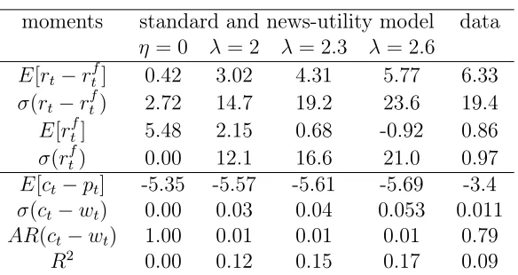
Table 2: Moments of the basic model
moments standard and news-utility model data
η= 0 λ= 2 λ = 2.3 λ= 2.6
E[rt−rft] 0.42 3.02 4.31 5.77 6.33 σ(rt−rtf) 2.72 14.7 19.2 23.6 19.4 E[rtf] 5.48 2.15 0.68 -0.92 0.86
σ(rft) 0.00 12.1 16.6 21.0 0.97
E[ct−pt] -5.35 -5.57 -5.61 -5.69 -3.4 σ(ct−wt) 0.00 0.03 0.04 0.053 0.011 AR(ct−wt) 1.00 0.01 0.01 0.01 0.79
R2 0.00 0.12 0.15 0.17 0.09
Value-weighted CRSP returns are displayed annualized and in percentage terms. The quarterly moments for the consumption-wealth ratio and predictability regression (rt+1 =α+β(ct−wt) +δrtf) are taken from Lettau and Ludvigson (2001) table II and III.
model is a long-run phenomenon and thus implies counterfactually high correlations between consumption growth and asset returns at longer horizons. Moreover, the auto-correlation of returns is negative in the model as opposed to around zero in the data.27
Finally, in table 3 I display the moments for a slight increase in θ, γ, and η to give a quantitative idea of the parameters’ implications.
The consumption-wealth ratio. The model’s simulated consumption-wealth ratio reflects the prior theoretical results. First, the consumption-wealth ratio is lower than in the standard model and exhibits variation. As consumption equals dividends in the classical Lucas-tree model and there is no labor income, the values are difficult to com-pare with the data. However, the corresponding values in Lettau and Ludvigson (2001) are displayed as an illustration. Both the standard and news-utility model roughly match the level of the consumption-price ratio, but the standard model mispredicts its variation whereas the news-utility model’s predicted variation is roughly in line with the data.28
However, the news-utility consumption-wealth ratio is i.i.d. whereas Lettau and Ludvigson (2001) find relatively high persistence.
The predictability properties compare quite favorably. The model is able to gener-ate predictability in quarterly returns yieldingR2 values of approximately 10% to 17%. Lettau and Ludvigson (2001) emphasize the medium-run predictive power of the aggre-gate consumption-wealth ratio. The authors obtain R2 values for quarterly returns of 9% and of 18% for annual excess returns.29
Lustig, Nieuwerburgh, and Verdelhan (2012)
27
Although, the aggregation to annualized frequency seems to introduce some spurious correlation as can be seen in the standard model’s moments.
28
Moreover, the consumption-wealth ratio cannot be used to forecast consumption growth, which is in line with the empirical findings in Lettau and Ludvigson (2001).
29
elaborate on the volatility of the consumption-wealth ratio and the return on the con-sumption claim. As noted by Hirshleifer and Yu (2011), traditional leading asset-pricing models have difficulty matching the volatility of the consumption-wealth ratio and the return on the consumption claim, because they rely on a volatile dividend process, and the only variation in the consumption-wealth ratio stems from heteroskedasticity in consumption growth. I can confirm this finding; using the return on the consumption claim, theR2 in the habit-formation model of Campbell and Cochrane (1999) is merely 1.6% and the R2 in the long-run risk model of Bansal and Yaron (2004) is just 2.9%.
Moreover, in figure 3 in appendix A I plot the simulated deviations of the news-utility, standard, habit-formation, and long-run risk consumption-wealth ratio and com-pare these with the annualdcay data provided by Lettau and Ludvigson (2005). For the habit-formation and long-run risk model I use the calibration of Campbell and Cochrane (1999) and Bansal and Yaron (2004) to then aggregate the consumption and wealth time series. Moreover, I feed in the deviations in log consumption growth ∆c−12µc of the d
cay data. As can be seen, news-utility introduces considerably more rapid variation in the consumption-wealth ratio than the standard model or the model augmented with long-run risk, but much less variation than the habit-formation model. While, the long-run risk consumption-wealth ratio appears to be too smooth and habit-formation wealth ratio too variable, the news-utility variation in the consumption-wealth ratio matches the dcay data quite well. Although it is disputable to compare the dcay data to the simulated data of a Lucas-tree model, I conclude that the rapid variation is supported by the data.30
At first blush, the model’s asset pricing implications appear to be mixed. News util-ity raises the equutil-ity premium and its volatilutil-ity to historical levels even though I omit a separate dividend process. Moreover, the variation in substitution motives generates strong variation in the consumption-wealth ratio and predictability in returns, match-ing the data better than leadmatch-ing asset-pricmatch-ing models. However, the model predicts excessive volatility in the risk-free rate, which I address in the following section.
5
Extensions
Motivation. The news-utility model’s most important shortcoming is the large pre-dicted variation in the risk-free rate. Nevertheless, I want to take the predictions of
θ,λ, or increasingγ.
30
Greenwood and Shleifer (2012) compare a variety of survey data on stock market expectations with the predicted expected returns of leading pricing models. The authors show that leading asset-pricing models implied expected returns do not correlate highly with the survey evidence on expected returns. In particular, the dcay model of Lettau and Ludvigson (2001) fits the survey data better than the habit-formation and long-run risk models do. I can confirm this finding using the American Association of Individual Investors Sentiment Survey and also find that the news-utility model is more positively correlated with the survey data than the habit-formation, long-run risk, models or thecayd
the evidence-based utility specification seriously and believe that people are very un-willing to substitute consumption intertemporally in some states of the world. The most important evidence is credit-card borrowing or pay-day loans. However, there may be forces at work that offset the effects on the aggregate risk-free rate. What would a consumption process look like which features an almost constant risk-free rate? An adverse shock to contemporaneous consumption growth has to be associated with an adverse prediction about future consumption growth to keep the risk-free rate low. Thus, the model’s risk-free rate process will become more smooth if low values ofεtare associated with a decrease inµc or an increase inσc. Variation in the agent’s expected consumption growth µc has been exploited by Bansal and Yaron (2004) and termed long-run risk. Variation in the agent’s expected volatility of consumption growth has been exploited by Campbell and Cochrane (1999) and Bansal and Yaron (2004).31
In section 5.1, I reverse-engineer variation in expected consumption growth and its volatility to offset the effect of the variation in the agent’s intertemporal smoothing incentives on the risk-free rate. An adverse shock to consumption growth today is then associated with low consumption growth but high volatility in the future. There exists empirical evidence for countercyclical variation in economic uncertainty, or con-sumption volatility.32
The empirical evidence on excess sensitivity suggests that there exists positive autocorrelation in consumption growth. However, it turns out that the variation in the agent’s smoothing incentives require variation in the agent’s expected consumption growth that is too large to be consistent with aggregate consumption data, because the variation in consumption volatility appears to be too weak to significantly affect the strong first-order variation in the agent’s risk-free rate. As another alterna-tive, I extend the model to account for time-variant disaster risk to smooth out the risk-free rate in section 5.2. Time-variant disaster risk is a very powerful device under news-utility preferences because they feature left-skewness aversion: The news-utility agent hates the left tail and thus disaster risk. It turns out that time-variant disaster risk is powerful enough to successfully offset the variation in the risk-free rate. More-over, Barro (2006) provides compelling evidence for the existence of a small probability of economic disaster.
It is important to note that introducing another source of variation does not
elim-31
Campbell and Cochrane (1999) specify heteroskedasticity in consumption growth to make the risk-free rate exactly constant.
32
inate the variation in substitution motives; it merely offsets its effects on the risk-free rate. Moreover, the extended models feature two sources of variation: The news-utility variation in substitution motives and heteroskedasticity in consumption growth or time-variant disaster risk. While the first source of variation concerns intertemporal substi-tution, the latter work via variation in the price of risk.
5.1
Time-variant consumption growth and volatility
Setup. A decrease in expected consumption growth µc or an increase in expected volatility σc make the agent consume less and save more. Thus, if an adverse shock is associated with a decrease in expected consumption growth or an increase in ex-pected volatility the agent’s intertemporal substitution effects on the risk-free rate will be partially offset. Let consumption growth be given by log(Ct+1
Ct ) = µt+σtεt+1 with
µt+1 =µc+νµ(µt−µc) + ˜µ(εt+1) +ut+1, ut+1 ∼(0, σ2u), andµ˜(εt+1) = ¯µ(log(1−ρtρ+1t+1)− E[log(1−ρt
ρt )]). Moreover, σ
2
t+1 =σc2 + ˜σ(εt+1) +νσ(σt2 −σc2) +wt+1, wt ∼ (0, σ2w), and
˜
σ(εt) = ¯σ(0.5−F(εt)). The variation in σ˜(εt+1) aims to reflect the variation in the ho-moskedastic consumption-wealth ratio, because heteroskedasticity is intended to offset the general-equilibrium impact on the risk-free rate. Note that σt is a Markovian pro-cess, increases in the event of an adverse shock and is characterized by a shape similar to the consumption-wealth ratio determined by the variation in intertemporal substitution motives. Moreover, the conditional expectation of economic volatility is characterized by an AR(1) process with persistenceνσ. µt is chosen to fine-tune the remaining vari-ation in the risk-free rate. The functional form ofµ˜(εt) is reverse-engineered such that ifµ¯ = 1and νµ= 0 the variation in the risk-free rate brought about by the variation in the price-consumption ratio will be exactly offset, as can be seen in equation (11). If
νµ >0the conditional expectation of consumption growth is characterized by an AR(1) process with persistence νµ. The model’s simple structure is unaffected by variation in expected consumption growth and derived in appendix C.
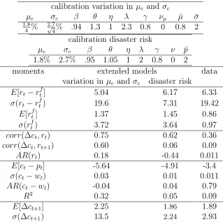
Time-variant consumption growth and volatility: Calibration and moments.
a second channel that offsets the impact on the risk-free rate. If νσ > 0, a positive shock to economic volatility today implies high volatility in the future because the heteroskedasticity process is autocorrelated. Then, the size of the excess returns will be autocorrelated and the model is able to generate autocorrelation in the returns and long-horizon predictability.33
However, µc, σc, and µ˜(·) jointly determine the moments of the annualized con-sumption growth process, which I also display in table 4 following Bansal and Yaron (2004). Unfortunately, the required variation inµ˜(·) significantly changes the moments of the annualized consumption growth process which then fails to match the data even if lower levels for both µc and σc are chosen. The annualized standard deviation of the simulated consumption process should be at most 3.5%. This value is far exceeded because of the extent of variation in expected consumption growth required to smooth out 80% of the variability of the risk-free rate.
5.2
Time-variant disaster risk
Setup. An increase in the probability of disaster makes the agent value a unit of safe consumption more highly. Thus, if adverse shock realizations of the world are associated with disaster risk the risk-free rate smooths out. Thus, I introduce a small time-variant probability of disaster according to Barro (2006, 2009). In each period t, there is a probabilitypt that a disaster occurs in periodt+ 1in which case consumption drops byd percent. Thus, consumption growth is given bylog(Ct+1
Ct ) =µc+εt+1+vt+1
with εt+1 ∼ N(0, σc2) and vt+1 = log(1−d) with probability pt and zero otherwise. I assume thatεt+1andvt+1are independent. The simple process governing the variability in disaster risk is pt+1 = p+ ν(pt − p) + ut+1 + ˜g(εt+1) with ut+1 ∼ N(0, σu2) and
˜
g(εt) =pp¯(0.5−F(εt)). Note that pt is a Markovian process, increases in the event of an adverse shock, and is characterized by a similar shape as the consumption-wealth ratio determined by the variation in intertemporal substitution motives. Moreover, the conditional expectation of disaster risk is characterized by an AR(1) process with persistence ν. The model’s simple structure is unaffected by the addition of disaster risk and derived in appendix D.
The news-utility agent is more affected by the probability of disaster than the stan-dard agent, because the news-utility agent dislikes disaster risk more. The utility func-tion’s gain-loss component over news is inspired by prospect theory. Classical prospect
33
Koszegi and Rabin (2007) find that news utility causes variation in risk attitudes. In proposition 1, the authors state that the agent becomes less risk averse when moving from a fixed to a stochastic reference point. With a stochastic reference point, a gamble does not appear as daunting, because some potential losses were previously expected. Thus, the equity premium in periodt depends negatively onσt−1, because it is determined by the price of risk, i.e., ECovt[Mt(tM+1t]+1σt,R(Rtt+1+1)), which varies with σtand
σt−1. If high volatility is expected,ρtis less steep and thus less responsive to a shock to consumption
growth, which tends to reduce the required equity premium. Hence, news-utility preferences introduce two sources of variation in the price of risk and thus the required equity premium: The price of risk varies with economic volatilityσt as in the standard model. Furthermore, for any givenσt, the price

![Figure 2: Annualized expected risky Et[Rt+1] and risk-free returns Rft+1 in the news-utility and standard models and annualized equity premium Et[Rt+1] − Rft+1 in thenews-utility and standard models](https://thumb-us.123doks.com/thumbv2/123dok_us/7792287.726417/34.612.153.453.394.637/annualized-expected-utility-standard-annualized-thenews-utility-standard.webp)