Munich Personal RePEc Archive
Assessment of Performance of
Correlation Estimates in Discrete
Bivariate Distributions using Bootstrap
Methodology
Tsagris, Michail and Elmatzoglou, Ioannis and C. Frangos,
Christos
University of Nottingham, Zeincro, Technological Educational
Institute of Athens
3 January 2012
Online at
https://mpra.ub.uni-muenchen.de/68057/
Assessment of Performance of Correlation Estimates in
Discrete Bivariate Distributions using Bootstrap
Methodology
Michael Tsagris1, Ioannis Elmatzoglou2, Christos C. Frangos3
1School of Mathematical Sciences, University of Nottingham, UK
2Zeincro S.A., Athens, Greece
3Department of Business Administration, Technological Educational Institute of Athens,
Greece
Corresponding author:
Michael Tsagris
School of Mathematical Sciences, Division of Statistics
University of Nottingham
University Park, Nottingham NG7 2RD
United Kingdom
Tel.: +44 (0) 7503242099, Fax: +44 (0) 115 95 13837
ABSTRACT
Little attention has been given to the correlation coefficient when data come from discrete or
continuous non-normal populations. In this paper we considered the efficiency of two correlation
coefficients which are from the same family, Pearson’s and Spearman’s estimators. Two discrete
bivariate distributions were examined, the Poisson and the Negative Binomial. The comparison
between these two estimators took place using classical and bootstrap techniques for the construction of
confidence intervals. Thus, these techniques are also subject to comparison. Simulation studies were
also used for the relative efficiency and bias of the two estimators. Pearson’s estimator performed
slightly better than Spearman’s.
1. INTRODUCTION
Bootstrap and jackknife are well-known resampling methodologies for obtaining
nonparametric confidence intervals of a parameter. In most statistical problems one needs an
estimator of an unknown parameter of interest as well as some assessment of its variability. In
many such problems the estimators are complicated functionals of the empirical distribution
function and it is difficult to derive trustworthy analytical variance estimates for them.
Bootstrap (Efron, 1979, 1982, 1987) and jackknife (Miller, 1974) use straightforward but
extensive computing to produce reliable indications of the variability of an estimator. For the
justification of bootstrap with regard to the foundation of its theoretical basis we have to say
the following. The primary objective of this technique is to estimate the sampling distribution
of a statistic. Essentially, bootstrap is a method that mimics the process of sampling from a
population, like one does in Monte Carlo simulations, but instead drawing samples from the
observed sampling data. The tool of this mimic process is the Monte Carlo algorithm of Efron
(1979).
This process is explained properly by Efron and Tibshirani (1993), who also noted that
bootstrap confidence intervals are approximate yet better than the standard ones.
substitute for precise parametric results, but rather a way to reasonably proceed when such
results are unavailable.
Bootstrap is in line with the general direction which Rao has imposed for the statistical
discipline and is “to extract all the possible information from the data” (Rao, 1989). One,
however, can pose the following question: Why is the bootstrap estimate of variance
converging to the true variance? The answer is the following: The strong law of large
numbers implies that Sˆ2 S2
B almost surely as B, in which case B stands for the
number of bootstrap samples and S stands for the standard deviation. What is the permissible
necessary value of B? In this respect we use the reference of Booth and Sarkar (1998). These
researchers suggested that a choice between 200 and 800 is satisfactory for the estimation of
the standard error and thus for the construction of confidence intervals. With the great power
of computing today we can have a safe choice of B equal to 1000, although Chernick (2008)
suggests using B=100,000.
In this paper we have not used powerful bootstrap variations like the partial likelihood
approach and bootstrap calibration. These methods have been proposed by Davison et al.
(1992), Beran (1987), Loh (1987) and Efron and Tibshirani (1993).
The choice for study of correlation coefficients was due to the fact that not much attention has
been given to this parameter and most of the authors who have dealt with it used bivariate
normal or log-normal distributions. Efron and Tibshirani (1993) used bootstrap techniques to
estimate the standard error of (Pearson’s) rho in the bivariate normal distribution. They also
showed that the non-parametric delta method can be badly biased. Dolker et al. (1982)
pointed out some possible problems in the correlation coefficient for very small sample sizes.
The probability of such discrepancies (same bivariate vectors) is very low in our case.
Rasmussen (1987) worked on the estimation of Pearson’s correlation coefficient for normal
and non-normal distributions and saw that Pearson’s coefficient is robust to deviations from
the normality assumption. Hall et al. (1989), Frangos and Schucany (1990) and Lee and
continuous bivariate distributions, and mainly the normal distribution, were examined. There
are more examples of researchers who studied the correlation coefficient. For instance, Young
(1988) used the Gaussian, log-normal and t distributions, and Hall et al. (1989) also used
normal and log-normal distributions but with small sample sizes (n=8, 10 and 12). Lunneborg
(1985) used a sample of the famous LSAT data for which the distribution is close to bivariate
normal.
In this paper the correlation coefficient is examined in the bivariate Poisson and Negative
Binomial distributions. The disadvantage of these two bivariate distributions is that the
correlation coefficient is strictly non negative. However, the bivariate Poisson has a nice
property. When the covariance term is zero and hence the correlation coefficient is zero, we
end up with two independent Poisson variates (Kawamura, 1973). Both of these discrete
distributions have a wide variety of applications, such as sports (Karlis and Ntzoufras, 2003,
2005) or medicine (hospital and doctor visits for instance). For more information about the
applications of the Poisson or Negative Binomial models one can also read the two papers by
Greene (2007).
Section 2 of this paper describes the Normal, Basic, Percentile, ABC, Studentized and the
accelerated bootstrap (BCa) methods, using both the positive and negative jackknives to
estimate the acceleration constant a. Section 3 describes the Classical method of constructing
confidence intervals for the correlation coefficient. Section 4 describes some characteristics of
these confidence intervals. The comparison is accomplished by an extensive simulation study
in which the properties of these intervals are examined in sections 4 and 5. All algorithms
were implemented in R 2.9.0 and the package “boot” was used.
2. NON PARAMETRIC BOOTSTRAP CONFIDENCE INTERVALS
Let X1, X2,,....,Xn, be n independent and identically distributed random variables from an
unknown probability distribution Fθ(x). Let Fˆ be the empirical distribution function, having
random samples X1*,X2*,...,Xn* with replacement from Fˆ and then calculates
)
,...,
(ˆ
ˆ
* *1 *
n
as an estimate of θ. After B replications of this process, one has anempirical distribution of
ˆ
*b
(b=1,…,B) values, which serves as an estimate of the unknownsampling distribution of
ˆ
. Following Efron (1987), to construct nonparametric confidenceintervals for θ via the Percentile method (PM), one uses the 100α and 100(1-α) percentiles of
the bootstrap distribution of θ. The 100(1-2α)% central confidence interval for θ is given by
)] 1 ( ˆ ), ( ˆ
[G 1 a G 1 a
B
B
(2.1)with
G
Bt
bB
t
}
ˆ
{
#
)
(
ˆ
*
(2.2)
being the estimated bootstrap distribution function.
Normal method (or standard confidence interval) has the known form of
)] ˆ ( ˆ
), ˆ ( ˆ
[
(1 )
( )
SE SE (2.3)where SE(
ˆ) is a reasonable estimate of the standard error of
ˆ
based upon theˆ
*b
(b=1,…,B) values and () 1() can be obtained from the tables of standard normal
distribution.
The bias-corrected method with acceleration constant α, (BCα), introduced by Efron and
Tibshirani (1986) and discussed in detail by Efron (1987), is a procedure for improved
confidence intervals for problems where there exists a monotone transformation g such that
) ˆ ( ˆ
g and
g(
) satisfy the approximationˆ
~
(
,
2),
0
N
Z
where. 1
This yields the 100(1 – 2α)% confidence interval
]))}
1
[
(
(
])),
[
(
(
{
1
1
G
Z
G
Z
Bwhere ) ˆ ( ˆ 1 ˆ ˆ ] [ 0 0 0
(2.5)
Note that Bias Correction (BC) intervals are BCα, with ˆ 0 and they further reduce to PM
when Zˆ0 0. The bias correction Zˆ0 is calculated using the formula } .
ˆ ˆ { # Zˆ 1 b*
0
How does one findˆ ? Efron (1987) showed that for one-parameter families,
f
(
T
),
ofsampling distributions of
T =
ˆ
, a good approximation is)) T ( i( SKEW 6 1
ˆ ˆ
(2.6a)
where SKEWˆ(i(T)), is the skewness of Fisher’s score function
)
(
ln
)
/
(
)
(
T
f
T
i
at
ˆ
.
He also proposed that for data from an arbitrarydistribution
F
and
t
(
F
)
the constant ˆ is reasonably well approximated by2 / 3 n 1 i 2 i n 1 i 3 i ) I ( ) I ( 6 1 ˆ
(2.6b)
where
I
i is the influence function of the functional t at the pointx
i. Two different finitesample estimates of the influence function
I
i are investigated here: the negative jackknife:
)
(
I
)]
,...,
,
,...,
(ˆ
)
,...,
(ˆ
)[(
1
(
1 n 1 i 1 i 1 ni
n
x
x
x
x
x
x
I
(2.7a)and the positive jackknife
(
I
)
:
)].
,...,
(ˆ
)
,
,...,
(
ˆ
)[(
1
(
1 n i 1 ni
n
x
x
x
x
x
The ABC method (stands for approximate bootstrap confidence intervals) is a method of
approximating the BCα interval endpoints analytically, without using any Monte Carlo
replications at all (Efron and Tibshirani, 1993). It requires the resampling vector
) ,..., ,
( * *
2 * 1 *
n
P P P
P which consists of the proportions
n
x
x
n
N
P
j ii i
}
{
#
/
* **
*
, i=1,2,…,n. Therefore, the statistic e.g.
n
i i
A 1
* *
ˆ
is expressedas ˆ .
1 * *
n
i i i
A P
The calculation of the confidence limits requires the calculation of someempirical influence components and of the acceleration constant which is again calculated as
1/6 times the standardized skewness of the empirical influence components.
Following Abramovitch and Singh (1985), as well as Loh (1987), we investigate a studentized
statistic that is resampled to yield bootstrap confidence intervals for . The approximation of
the distribution of (
ˆ
)/SE(
ˆ) was carried out using the bootstrap distribution of thestudentized pivotal quantity (SPQ), namely
), ˆ ( / ) ˆ ˆ
( * *
*
SE
t (2.8)
where SE(
ˆ) is the square root of the estimated Var(
ˆ). Denote by Gs(t)#{tb* t}/Bthe bootstrap distribution of the studentized quantity t*. The bootstrap confidence interval has
the form:
)]
ˆ
(
)
(
ˆ
),
ˆ
(
)
1
(
ˆ
[
1
1
G
s
a
SE
G
sa
SE
(2.9)The estimator for the standard error (the denominator in 2.8) of Pearson’s correlation
coefficient is (1
ˆ2)/ n3. The assumption of normality is necessary in order for thisestimator to hold true, even though this assumption is not realistic at all. As for Spearman’s
correlation coefficient, a different approach was used. Instead of performing a second
bootstrap in each bootstrap sample to estimate the standard error we estimated this standard
correlation coefficient we generated 1000 pairs, estimated the Spearman correlation
coefficient and then calculated the standard deviation of these values.
The Basic method is a combination of the Percentile and Studentized methods. Instead of
trying to find the empirical distribution of
ˆ
*b
(b=1,…,B), this method finds the empiricaldistribution of
ˆ
*
.ˆ
b Note that this statistic is the same as in the studentized method with
the only difference being that the denominator (standard error of
ˆ)
is set equal to one). Theconfidence interval for the parameter is given by the formula:
)], ( ˆ ˆ 2 ), 1 ( ˆ ˆ 2
[ G1 a G1 a
(2.10)where
G
1(
t
)
B is the same as in (2.2).
3. CLASSICAL CONFIDENCE INTERVAL
The classical confidence interval (Fisher’s method) for the correlation coefficient is extracted
through the Z-transform,
)
tanh
(
).
1
1
ln(
5
.
0
1
The confidence interval for z is
[
ˆ
(
),
ˆ
(
)]
[
L
,
U
]
where
ˆtanh1(r) and
2(
)
1
/(
n
3
).
It follows that the confidence interval for the correlation coefficient is given by
)]
1
/(
)
1
(
),
1
/(
)
1
[(
2
2
2
2
e
Le
Le
Ue
U
(3.1)The above formula was applied to both coefficients, since normality was assumed.
4. SOME CHARACTERISTICS OF THE ABOVE CONFIDENCE INTERVALS The transformation respecting property allows us to construct confidence intervals for a
parameter, then transform the endpoints of the interval and end up with confidence intervals
for a transformation of the original parameter of interest. If, for instance, we have constructed
by squaring the endpoints of the initial confidence interval. The accuracy term refers to the
rate of convergence, of the coverage probability, to the desired level of coverage. A central
(1-2α) confidence interval is supposed to have probability α of not covering the true value of
from above and below. In the case of a sample this probability is equal to α+n c or α+
n
c
for some constant
c
.
In the first case the fraction goes to zero at rate 1/n, whereas in thesecond case it goes to zero at rate
1
/
n
.
We refer to the first case with the term second-orderaccuracy and with the term first-order accuracy to the second case.
The Normal (or Standard) method is known to be neither transformation respecting nor
second-order accurate. Percentile and Basic methods are transformation respecting, but not
second-order accurate. The BCα method is both transformation respecting and second-order
accurate. The Studentized method is second-order accurate but not transformation respecting.
If interest lies in estimating the correlation coefficient of the bivariate normal distribution then
Fisher’s transform works quite well. The problem arises in non normal populations like in our
case. The drawback of not using a transformation is that one can end up with an interval not
satisfying the range restriction. We did not use any transformation in the Studentized method
and the result was obvious for small sized samples (n=10). The interval was larger than the set
of permissible values for the correlation coefficient since this method is not range-preserving.
The ABC method is both second-order accurate and transformation respecting. One could
also say that since the Studentized method performs double bootstraps when the denominator
is not known (in our case it is known), it needs more computational effort. On the other hand
the ABC method requires far fewer replications than its counterpart (BCα) needs. More
information on the advantages and disadvantages of the various bootstrap methods can be
found in Hall (1988), Efron and Tibshirani (1993), and DiCiccio and Efron (1996).
5. SIMULATIONS AND RESULTS
A simulation study was performed as follows: 2000 independent samples of size 10, 20, 50
Each time we estimated the correlation coefficient using the two estimators and for the
bootstrap confidence intervals construction, the number of bootstrap samples was set equal to
B=1000. Bivariate Poisson variates were generated according to the method described in
Morgan (1984). The probability mass function of the bivariate Poisson is given by the
following formula:
)]
(
exp[
!
)!
(
)!
(
)
,
(
1 2 3) , min( 0 3 2
1
yx x y
y
x
y
Y
x
X
P
(5.1)Parameters
1 and
2 were fixed at 0.5 and 1, respectively. What did not remain constantwas the parameter of the covariance term
(
3).
The correlation between X and Y is given bythe following formula
) )(
( 1 3 2 3 3
(5.2)
For the selected values of the correlation, 0.25, 0.5, 0.75 and 0.9, the values of the covariance
were 0.24, 0.73, 2.22 and 6.71, respectively.
Random values from a Negative Binomial distribution can be generated in many ways, by the
process of compounding a Poisson distribution as in the univariate case or with the help of
two univariate Negative Binomial variates and one univariate Binomial variate. These
methods are better described in Kocherlakota and Kocherlakota (1992). In this paper the
method of rejection sampling was used. For more information on the computer generation of
the bivariate Negative Binomial distribution one can also look at Loukas and Kemp (1986).
The distribution function is given by the formula
r y
x
p
p
p
p
y
x
r
y
x
r
y
Y
x
X
P
(
1
)
!
!
)!
1
(
)!
1
(
)
,
(
1 2
1
2
(5.3)The correlation between X and Y is given by the following formula
) 1 )( 1
( 1 2
2 1 p p p p
The values of the correlation coefficients were set equal to 0.25, 0.5 and 0.75. The
confidence intervals for the correlation coefficient valued 0.9 in the bivariate Negative
Binomial distribution were not computed due to computational difficulties. We set the
parameters
p
1 andp
2 to the values of (0.1393, 0.2786), (0.2287, 0.4574) and (0.2898,0.5796), respectively. The number of successes (r) was set equal to 5. Bootstrap confidence
intervals with coverage probability 1-2α=
n =0.95 for the correlation coefficient werecalculated with each of the eight methods described above. Tables l & 3 and 2 & 4 present the
expected coverage and average length of the confidence intervals for the Poisson and
Negative Binomial cases, respectively.
5.1 Pearson's estimator
Tables 1 and 2 summarize the results of the simulations for Pearson’s estimator. In the
Poisson distribution, when the values of the correlation coefficient are less than or equal to
0.5 and the sample size is equal to 10, the average length exceeds unity. The Studentized
method provides good confidence intervals in general (amongst the ones compared) but with
the cost that the average length is the largest in all cases. The average length exceeded the
length of the interval of possible values of the correlation coefficient. Since the pivotal
quantity used here was not the same as Fisher’s, this problem occurs naturally. However, as
the sample size increases the estimated coverage probability reaches the nominal level of 0.95
faster and better than in the other methods. The Normal and Basic methods did not work very
well in general. As correlation and sample size increase, they tend to provide better results.
The average lengths are in accordance with the lengths of the other methods, but this is not
true for the estimated coverage. BCα and Fisher’s based intervals are the most stable in
general. No matter the value of the correlation and the sample size, they tend to produce
stable results in terms of coverage probabilities. The ABC and Percentile methods perform
the true coverage probability, but not more than Normal and Basic methods. The Percentile
[image:13.595.101.494.219.703.2]method leads to similar conclusions.
Table 1. Estimates of the actual coverage,
n
0
.
95
in percent (first line) and the expected length, (second line): Poisson distribution using Pearson’s formulaCorrelations Sample sizes
Methods
Normal Basic Percentile ABC BCα(I-) BCα(I+) Studentized Fisher’s
ρ=0.25
n=10 85.4
1.154 76.6 1.136 89.6 1.136 90.45 1.128 92.8 1.188 93.6 1.194 98.4 -* 94.2 1.126
n=20 87.35
0.826 82.7 0.819 91.85 0.819 91.2 0.794 92.95 0.826 93.5 0.829 95.8 1.064 93.15 0.829
n=50 90.95
0.534 88.95 0.533 93.0 0.533 92.4 0.526 92.5 0.534 92.85 0.534 94.15 0.584 92.9 0.534
n=100 91.8
0.386 90.4 0.386 92.85 0.386 93.15 0.383 92.65 0.387 93.05 0.386 93.6 0.404 92.9 0.386 ρ=0.5
n=10 84.35
1.007 75.4 0.987 90.1 0.987 87.74 0.987 92.35 1.053 93.8 1.077 96.55 - 92.75 1.077
n=20 88.55
0.683 82.5 0.677 92.3 0.677 91.4 0.666 93.45 0.6927 94.2 0.701 95.85 0.875 93.4 0.701
n=50 91.7
0.44 89.2 0.44 92.65 0.44 92.65 0.439 93.1 0.444 93.4 0.446 94.55 0.482 92.45 0.446
n=100 92.5
0.316 91.1 0.316 93.6 0.316 93.6 0.316 93.45 0.317 93.45 0.317 94.45 0.33 92.75 0.317 ρ=0.75
n=10 86.85
0.692 76.0 0.672 90.8 0.672 87.995 0.696 93.4 0.747 94.15 0.798 96.45 - 93.35 0.798
n=20 87.75
0.424 81.45 0.419 90.95 0.419 90.8 0.427 92.05 0.4407 92.7 0.455 93.7 0.54 92.75 0.455
n=50 91.55
0.263 88.15 0.263 93.55 0.263 93.45 0.267 93.45 0.269 93.75 0.272 95.0 0.285 92.85 0.272
n=100 92.5
0.187 89.95 0.187 93.65 0.187 92.9 0.19 93.0 0.19 93.25 0.191 93.55 0.195 92.15 0.191 ρ=0.9
n=10 87.7
0.372 73.3 0.35 89.4 0.35 84.2 0.377 91.6 0.419 92.5 0.473 95.25 - 93.15 0.473
n=20 88.45
0.2 81.7 0.197 91.75 0.197 90.2 0.208 91.65 0.214 92.1 0.225 93.5 0.25 93.8 0.225
n=50 91.5
0.116 86.05 0.116 93.7 0.116 93.65 0.12 93.5 0.12 93.65 0.122 94.4 0.125 93.4 0.122
n=100 92.6
0.082 90.7 0.082 93.55 0.082 93.85 0.084 94.4 0.084 94.35 0.085 94.15 0.085 92.9 0.085
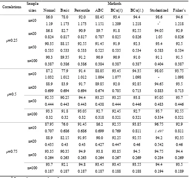
Table 2. Estimates of the actual coverage,
n
0
.
95
in percent (first line) and the expected length, (second line): Negative Binomial distribution using Pearson’s formulaCorrelations Sample sizes
Methods
Normal Basic Percentile ABC BCα(I-) BCα(I+) Studentized Fisher’s
ρ=0.25
n=10 86.0
1.19 78.0 1.173 92.0 1.173 88.45 1.151 93.4 1.209 94.4 1.218 98.6 -* 94.6 1.218
n=20 86.8
0.824 82.7 0.817 90.9 0.817 89.7 0.787 91.8 0.825 92.55 0.826 94.05 1.05 92.9 0.826
n=50 90.35
0.535 88.15 0.533 92.55 0.533 91.45 0.525 91.9 0.535 92.3 0.534 93.4 0.583 92.5 0.534
n=100 90.3
0.387 89.35 0.386 91.2 0.386 90.9 0.384 90.9 0.387 91.0 0.387 91.1 0.404 91.5 0.387 ρ=0.5
n=10 87.2
1.032 77.9 1.012 91.4 1.012 88.05 1.004 93.45 1.077 94.35 1.098 98.05 - 93.75 1.098
n=20 88.9
0.699 83.9 0.694 91.7 0.694 89.85 0.674 92.0 0.705 92.85 0.713 94.65 0.883 93.5 0.713
n=50 92.55
0.444 90.25 0.443 94.4 0.443 93.25 0.438 93.25 0.444 93.8 0.446 95.05 0.483 93.7 0.446
n=100 93.3
0.32 91.8 0.32 93.05 0.32 92.7 0.318 92.45 0.321 92.7 0.321 93.7 0.334 92.55 0.321 ρ=0.75
n=10 87.95
0.707 76.0 0.686 91.45 0.686 86.2 0.699 92.55 0.769 93.85 0.811 96.75 1.497 92.9 0.811
n=20 88.9
0.435 82.15 0.43 91.95 0.43 90.0 0.427 92.25 0.447 92.55 0.46 94.2 0.542 92.35 0.46
n=50 93.35
0.264 90.35 0.263 94.9 0.263 93.8 0.264 93.85 0.267 94.5 0.269 94.75 0.284 94.4 0.269
n=100 93.7
0.187 92.1 0.187 94.8 0.187 93.45 0.187 93.45 0.188 93.55 0.188 94.4 0.194 93.5 0.189
* Length greater than 2.
Similar conclusions are to be drawn in the bivariate Negative Binomial distribution case as
well. The Normal and Basic methods perform the same as before and as the sample size
increases from n=20 to n=50 the estimation of the coverage probability is closer to the desired
nominal level but the average length is not reduced by the same amount as before. The
Percentile method estimates the coverage to be more than 0.90 irrespective of the sample size
or the correlation value. The performance of the ABC method is about the same as before.
The stability of BCα and Fisher’s methods are also met in this case. Studentized confidence
intervals are more conservative; they overestimate the nominal level of 0.95 for small samples
Although these conclusions are drawn with respect to Pearson’s formula, similar conclusions
can be drawn when using Spearman's formula.
5.2 Spearman's estimator
Tables 3 and 4 summarize the simulation results for Spearman’s estimator. In the bivariate
Poisson case, when the values of the true correlation coefficient are less than or equal to 0.5
and the sample is of size 10, the average length of the 95% confidence intervals exceeds unity
except for the ABC method with a correlation equal to 0.5. The estimated coverage tends to
the nominal level as the values of the correlation and the sample size increase, but the
convergence seems to be faster as the true values of the coefficient increase rather than as the
sample size increases.
The Normal and Basic methods perform better with this non-parametric estimator and the
Percentile method works much better in comparison to the parametric estimator regardless of
the combinations of the sample size and the correlation coefficient values. The ABC method
shows a significant improvement also. The BCα methods and Classical method (Fisher’s
transform) work very well under any circumstances, which was also the case before.
However, BCα methods perform a little better using Spearman's estimator.
In contrast to Pearson's estimator, the Studentized method as applied in Spearman’s estimator
does not perform similarly. The coverage is approached for large samples only (from 50 and
above) and as the correlation increases the approach is better.
With Negative Binomial distribution, things are slightly different. The average length exceeds
unity in the same occasions as with the Poisson distribution. Normal and Basic methods using
this non-parametric estimator perform slightly better than using the parametric estimator. The
performance of the Percentile method is roughly at the same levels for both estimators, and so
is the ABC method. The results for BCα, Studentized and Fisher's methods are similar using
Table 3. Estimates of the actual coverage,
n
0
.
95
in percent (first line) and the expected length, (second line): Poisson distribution using Spearman’s formulaCorrelations Sample sizes
Methods
Normal Basic Percentile ABC BCα(I-) BCα(I+) Studentized Fisher’s
ρ=0.25
n=10 88.8
1.2039 80.6 1.1805 93.2 1.1805 89.92 1.1375 95 1.2239 95.2 1.2337 80.6 1.1805 94.2 1.2367
n=20 90.45
0.8442 86.9 0.8396 93.05 0.8396 90.7 0.7951 94.65 0.8541 94.8 0.8553 86.9 0.8396 92.75 0.8553
n=50 93.4
0.5337 91.85 0.534 94.5 0.534 92.35 0.5263 95.5 0.5368 95.55 0.5369 91.85 0.534 92.35 0.5369
n=100 94.05
0.3777 93.9 0.3786 94.95 0.3786 94.0 0.3845 95.3 0.3794 95.3 0.3794 93.9 0.3786 93.4 0.3794 ρ=0.5
n=10 86.0
1.0551 79.4 1.0395 91.6 1.0395 88.16 0.9861 92.4 1.0994 93.0 1.1196 79.4 1.0395 92.6 1.1196
n=20 91.5
0.7274 87.3 0.7222 94.2 0.7222 91.25 0.6735 95.3 0.7507 95.55 0.7537 87.3 0.7222 93.45 0.7537
n=50 94.05
0.4525 92.9 0.4519 95.45 0.4519 93.3 0.4381 95.7 0.4597 95.75 0.4599 92.9 0.4519 93.15 0.4599
n=100 94.15
0.3178 94.1 0.3181 94.6 0.3181 92.85 0.3181 94.7 0.3209 94.7 0.321 94.1 0.3181 92.1 0.321 ρ=0.75
n=10 88.4
0.7848 79.8 0.7686 92.6 0.7686 86.61 0.6805 93.0 0.8456 94.2 0.8847 79.8 0.7686 92.2 0.8847
n=20 91.15
0.4969 85.25 0.4919 94.75 0.4919 90.15 0.4296 93.9 0.5246 94.1 0.5307 85.25 0.4919 92.9 0.5307
n=50 93.45
0.2965 91.3 0.2955 94.3 0.2955 92.2 0.267 93.95 0.3063 94.0 0.3068 91.3 0.2955 93.0 0.3068
n=100 94.2
0.2058 93.6 0.2058 93.4 0.2058 93.3 0.1879 93.2 0.2097 93.15 0.2098 93.6 0.2058 92.9 0.2098 ρ=0.9
n=10 92.6
0.4985 80.0 0.4824 96.8 0.4824 86.48 0.3846 93.8 0.5548 95.0 0.6076 80.0 0.4824 94.0 0.6076
n=20 94.0
0.2924 86.9 0.2871 96.35 0.2871 90.15 0.209 93.8 0.3097 94.2 0.3172 86.9 0.2871 93.45 0.3172
n=50 94.3
0.1552 91.1 0.1541 94.85 0.1541 93.0 0.122 92.85 0.1601 92.9 0.1608 91.1 0.1541 93.25 0.1608
n=100 95.6
Table 4. Estimates of the actual coverage,
n
0
.
95
in percent (first line) and the expected length, (second line): Negative Binomial distribution using Spearman’s formulaCorrelations Sample sizes
Methods
Normal Basic Percentile ABC BCα(I-) BCα(I+) Studentized Fisher’s
ρ=0.25
n=10 84.6
1.2219 78.2 1.2034 90.0 1.2034 85.57 1.0786 92.6 1.2419 93.4 1.253 78.2 1.2034 93.0 1.253
n=20 90.8
0.8656 87.8 0.8601 94.15 0.8601 90.6 0.7859 95.35 0.8909 95.45 0.872 98.15 1.1189 93.3 0.872
n=50 92.85
0.5405 92.4 0.5402 93.95 0.5402 91.8 0.5265 94.4 0.5421 94.4 0.5422 92.4 0.5402 93.75 0.5422
n=100 91.35
0.3813 91.35 0.3822 91.6 0.3822 91.35 0.3822 91.8 0.3829 91.8 0.3829 91.35 0.3822 91.65 0.3829 ρ=0.5
n=10 89.7
1.1347 82.75 1.1169 95.6 1.1687 88.38 0.9877 95.8 1.1591 96.6 1.1802 82.75 1.1169 93.55 1.1802
n=20 92.45
0.7643 89.55 0.7593 95.05 0.7593 89.85 0.6816 95.1 0.7751 95.2 0.778 98.15 0.999 93.3 0.778
n=50 94.25
0.4671 94.0 0.4666 94.45 0.4666 92.15 0.4426 94.3 0.471 94.3 0.4713 94.0 0.4666 93.05 0.4713
n=100 93.8
0.3248 94.3 0.3251 92.55 0.3251 92.8 0.3251 92.05 0.3266 92.05 0.3267 94.3 0.3251 92.45 0.3267 ρ=0.75
n=10 93.85
0.8928 85.7 0.8743 96.8 0.8743 86.31 0.7222 96.15 0.9101 96.9 0.9482 85.7 0.8743 93.6 0.9482
n=20 95.25
0.5437 90.35 0.5388 96.3 0.5388 90.5 0.4364 95.3 0.5502 95.55 0.5567 90.35 0.5388 93.2 0.5567
n=50 95.6
0.3077 93.9 0.3071 94.5 0.3071 91.7 0.2654 94.1 0.3101 94.05 0.3107 93.9 0.3071 92.7 0.3107
n=100 95.45
0.2086 94.9 0.2084 93.35 0.2084 93.4 0.1875 92.95 0.2093 92.95 0.2095 94.9 0.2084 93.1 0.2095
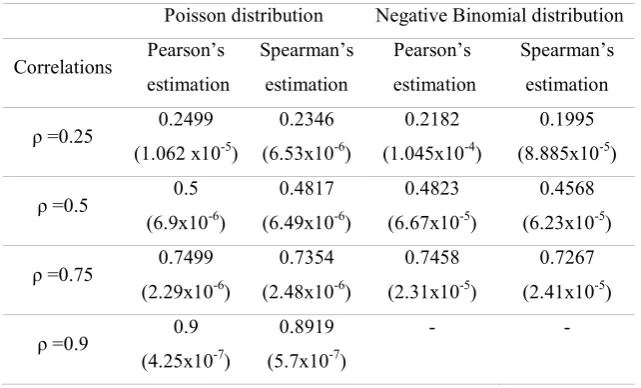
5.3 Examination of some properties of these two estimators under the given distributions The bias of the estimators is under examination in this section. We generated 1,000,000 pairs
of data from each distribution using the 4 chosen correlation values (0.25, 0.5, 0.75 and 0.9)
and estimated the correlation using both estimators. We repeated this procedure 1000 times.
Finally, the mean of the 1000 estimators was compared to the true correlation value and the
bias was extracted. The variance of these 1000 estimators was also calculated. The results are
shown in Table 5.
As seen from Table 5 in the Poisson case, Pearson’s estimator is asymptotically unbiased
these two estimators have in common is their asymptotic normality. The distribution of both
estimators for the sample examined was clearly non-normal (not even of symmetric form) and
that was evident from their confidence intervals. Furthermore, Pearson's estimator converges
to normality faster than his competitor’s estimator. This was apparent since this procedure
was repeated with 10,000 pairs of data and normality (using Shapiro's test) was rejected
[image:18.595.138.459.268.462.2]sometimes for Spearman's estimator, but never for Pearson's estimator.
Table 5. Estimated bias for large sample sizes (the variance is presented in parentheses)
Poisson distribution Negative Binomial distribution
Correlations Pearson’s estimation
Spearman’s estimation
Pearson’s estimation
Spearman’s estimation
ρ =0.25 0.2499 (1.062 x10⁻⁵)
0.2346 (6.53x10⁻⁶)
0.2182 (1.045x10⁻⁴)
0.1995 (8.885x10⁻⁵)
ρ =0.5 0.5 (6.9x10⁻⁶)
0.4817 (6.49x10⁻⁶)
0.4823 (6.67x10⁻⁵)
0.4568 (6.23x10⁻⁵)
ρ =0.75 0.7499 (2.29x10⁻⁶)
0.7354 (2.48x10⁻⁶)
0.7458 (2.31x10⁻⁵)
0.7267 (2.41x10⁻⁵)
ρ =0.9 0.9 (4.25x10⁻⁷)
0.8919 (5.7x10⁻⁷)
- -
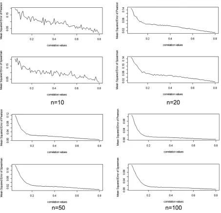
5.4 Comparison of the estimators in terms of the mean square error
MSE is a criterion used to assess at some degree the efficiency of an estimator and to compare
estimators. It is defined as the sum of the variance of the estimator and the squared bias of the
estimator.
In this section, we compared the estimators using a wider range of values for the covariance
parameter for each of the already studied sample sizes (n=10, n=20, n=50 and n=100). That is,
we used values for the correlation coefficient ranging from 0.05 to 0.95, each time increasing
by 0.01. The MSE for both estimators was estimated for all values using different sample
sizes each time for both distributions. For every value of the correlation and each sample size,
random values from each distribution were generated and the correlation coefficient was
and used for the extraction of the MSE. The results are shown in Figures 1 and 2 for the
[image:19.595.90.544.150.594.2]Poisson and negative Binomial, respectively.
Figure 1. Poisson distribution
It can be seen that MSE values are very close to each other. Approximately half of the time,
the difference between the MSE of Pearson’s and the MSE of Spearman’s estimator is
positive. Regardless of the sign of the difference, the maximum difference between them does
estimator is lower than that of Pearson’s estimator, but as the correlation increases, the
[image:20.595.90.544.124.561.2]opposite pattern occurs.
Figure 2. Negative binomial distribution 6. DISCUSSION
In this study an examination was performed of several bootstrap confidence intervals for the
correlation coefficient when the populations are discrete. The two bivariate distributions that
were examined were the Poisson and the Negative Binomial. Furthermore, two estimators
were compared--Pearson’s and Spearman’s formula. What was apparent was that as the
increases. The same is true with the sample size. As for the comparison of the confidence
intervals, the BCα family of confidence intervals exhibited great stability under all
circumstances. The same is true for Fisher’s transformation, regardless of the estimator used
(parametric or not).
MSE as a criterion for a further comparison of these two estimators showed that they produce
results that are very close. A further examination though showed that Pearson’s formula is
asymptotically unbiased, whereas its non-parametric alternative is not. In addition, the
parametric estimator tends to normality faster that the non-parametric estimator.
In our opinion, based upon the findings of the simulations we propose the use of Pearson’s
estimator instead of Spearman’s and the Fisher’s transform for confidence intervals
construction. The reason is that Fisher’s transformation is simpler than the Bcα, which also
performs very well in general.
There are still more bootstrap techniques for the correlation coefficient and certainly many
more bivariate distributions (discrete or continuous) whose correlation coefficients are to be
examined.
ACKNOWLEDGMENTS
The authors would like to thank Constantinos C. Frangos, University College London, for his
kind advice and support during the preparation of this manuscript. Additionally, we would
like to thank Thodoris Kypraios, Lecturer at the University of Nottingham, for reading a first
draft of this paper.
REFERENCES
Abramovitch, L. and Singh, K. (1985). Edgeworth corrected pivotal statistics and the
bootstrap. Ann. Stat. 13:116-132.
Booth, J. G. and Sarkar, S. (1998). Monte Carlo approximations of bootstrap variances. Am.
Stat. 52:354-357.
Chernick, M. (2008). Bootstrap Methods: A Guide for Practitioners and Researchers. New
Jersey: John Wiley & Sons
Davison, A. C., Hinkley, D. V. and Worton, B.J. (1992). Bootstrap likelihoods. Biometrika
79:113-130.
Davison, A. C. and Hinkley, D.V. (1997). Bootstrap methods and their application.
Cambridge: Cambridge University Press.
DiCiccio, T. J., and Efron, B. (1996). Bootstrap confidence intervals. Stat. Sci. 11:189-212.
Dolker, M., Halperin, S. and Divgi, D. R. (1982). Problems with bootstrapping Pearson
correlations in very small bivariate samples. Psychometrika 47:529-230.
Efron, B. (1979). Computers and the theory of statistics: Thinking the unthinkable. SIAM
Rev. 21:460-480.
Efron, B. (1982). The jackknife, the bootstrap, and other resampling plans. SIAM
CBMS-NSF Monograph 38.
Efron, B. (1987). Better bootstrap confidence intervals (with discussion). J. Am. Stat. Assoc.
82:171-200.
Efron, B. and Tibshirani, R. (1986). Bootstrap methods for standard errors, confidence
intervals, and other measures of statistical accuracy. Stat. Sci. 1:54-77.
Efron, B. and Tibshirani, R. J. (1993). An introduction to the bootstrap. Florida: Chapman
and Hall/CRC.
Frangos, C. C. and Schucany, W. R. (1990). Jackknife estimation of the bootstrap acceleration
constant. Comput. Stat. Data An. 9:271-281.
Greene, W. (2007). Functional Form and Heterogeneity in Models for Count Data. Found.
Trends Econom. 1:113-218
Greene, W. (2007). Functional forms for the negative binomial model for count data. Econ.
Hall, P. (1988). Theoretical comparison of bootstrap confidence intervals. Ann. Stat.
16:927-253
Hall, P., Martin, A. M. and Schucany, W. R. (1989). Better nonparametric confidence
intervals for the correlation coeffcient. J. Stat. Comput. Sim. 33 161-172.
Hall, P., DiCiccio, T. J. and Romano J. P. (1989).On smoothing and the bootstrap. Ann. Stat.
17:692-704.
Karlis, D. and Ntzoufras, I. (2003). Analysis of Sports Data Using Bivariate Poisson Models.
J. Roy. Stat. Soc. D-Sta. 52:381-393
Karlis, D. and Ntzoufras, I. (2005). Bivariate Poisson and Diagonal Inflated Bivariate Poisson RegressionModels in R. J. Stat. Softw. 14:Issue 10
Kocherlakota, S. and Kocherlakota, K. (1992). Bivariate discrete distributions. New York:
Marcel Dekker, Inc.
Lunneborg, E. C. (1985). Estimating the Correlation Coefficient: The Bootstrap Approach.
Psychol. Bull. 98:209-215.
Lee, W. and Rodgers, J. L. (1998). Bootstrap correlation coefficients using univariate and
bivariate sampling. Psychol. Methods 3:91-103.
Loh, W. Y. (1987). Calibrating confidence intervals. J. Am. Stat. Assoc. 82:155-162.
Loukas, S. and Kemp, C. D. (1986). The computer generation of bivariate binomial and
negative binomial random variables. Commun. Stat.-Simul. C. 15:15-25.
Miller, R. G. (1974). The jackknife: A review. Biometrika 6: 1-15.
Morgan, B. J. T. (1984). Elements of Simulation. London: Chapman and Hall.
Rao, C. R. (1989). Statistics and truth, putting chance to work. Burtonsville: International
Cooperative Publishing House.
Rasmussen, J. L. (1987). Estimating Correlation Coefficients: Bootstrap and Parametric
Approaches. Psychol. Bull. 101:136-139.
Tibshirani, R. (1988). Variance stabilization and the bootstrap. Biometrika 75:433-444.
Young, A. G. (1988). A Note on Bootstrapping the Correlation Coefficient. Biometrika