On the Existence of Quality Measures in Random Utility Models

Munich Personal RePEc Archive

On the Existence of Quality Measures in

Random Utility Models

Szczygielski, Krzysztof and Komisarski, Andrzej

CASE - Center for Social and Economic Research, University of

Lodz

30 October 2012

Online at

https://mpra.ub.uni-muenchen.de/42261/

On the Existence of Quality Measures in Random Utility

Models

Krzysztof Szczygielski (corresponding author)

CASE – Center for Social and Economic Research, Warsaw, Poland & Lazarski University, Faculty of Economics and Management

Al. Wilanowska 71/20 PL 02-765 Warsaw POLAND

[email protected]

Tel. 0048 501248601 Fax. 0048 22 8286069

Andrzej Komisarski

University of Lodz, Faculty of Mathematics and Computer Science, Lodz, Poland

Abstract

Random Utitly Models (RUMs) are a particularly convenient way of modelling product differentiation. In this paper we demonstrate that they can be used to examine the possibilities of creating quality measures from data on prices and sales volumes. We formulate conditions sufficient for the existence of quality measures in two broad families of RUMs: additive random utility models and pure vertical differentiation models.

JEL codes: C60, D43, L10, L13, L15

Keywords: quality measure, product differentiation, random utility models

1.Introduction

Random utility models have a wide range of applications in psychology, social science,

economics and natural science. They have also been subject to a considerable amount of

theoretical work. This work has been partly inspired by application problems, but is also, to a

large extent, ‘autonomous’ in nature (see the review by Marley (2002)). The problem we pose

and partly solve in this paper, belongs in the first category. It is motivated by our work on the

theory of consumer choice in a market with product differentiation.

One of the aspects of product differentiation is ‘quality’. Assuming the quality of individual

product varieties is unobservable, it might be tempting to infer it from data on sales volumes

and prices. Examples of such works are Khandelwal (2010) and Hallak and Schott (2011)

who create (and estimate) indicators of quality in foreign trade. Both papers use specific

demand functions (nested logit and a two-tier CES function, respectively), which can be

inverted so that the vector of qualities is isolated. The question we would like to ask is, when

is such an inversion possible in general? Or in other words: when can the quality measure be theoretically identified, given the vector prices and sales volumes?

It is particularly convenient to formulate this problem in terms of random utility theory. In

this line of RUM applications, the deterministic components of the conditional utility function

are interpreted as price and quality of the product variety, whereas the stochastic component

stands for consumers’ subjective tastes. We demonstrate that the conditions sufficient for the

existence of quality measures can be expressed in terms of the specification of the random

utility function and the distribution of the stochastic component.

The rest of the paper is structured as follows. In Section 2 we formulate the problem in strict

terms. In Section 3 we demonstrate the results for some broad classes of random utility

functions, while in Section 4 we offer conclusions.

2. Problem Formulation

Assume a market with a differentiated product wherein the demand for different varieties of

the product is a result of the aggregation of individual choices made according to a random

utility model (RUM). We use the notation by Anderson et al. (1992)1 to describe these choices

by the individual conditional indirect utility function:

(

, ,

)

i i i i

V =V p a

ε

(2.1)

1

– where V_i is the utility of a the consumer from consuming the variety (model) i of a differentiated good (i=1, ,n). V_i is a function of three variables: the price of the i-th model

i

p ∈R+, the quality of the model a_i∈R, and

ε

_i which is a random variable interpreted as the individual satisfaction of the consumer from buying the variety. By definition, p_i is

nonnegative. Function V is increasing in a_i and

ε

_i, and decreasing in p_i. Variable a_i

represents the vertical dimension of product differentiation while the random variable

ε

_i

represents the horizontal dimension. A special case of (2.1) is the additive random utility

model (ARUM):

( , )

i i i i

V =w p a +

ε

(2.2a)

where w:R2 R is decreasing in the first argument and increasing in the second argument; or, even more specifically a linear random utility model (LRUM):

i i i i

V = −p +a +

ε

(2.2b)

Regardless of the form of the V function, it is assumed that the consumer makes a discrete

choice, i.e. she chooses only one model of the n varieties available: the one that yields her the biggest utility V_i.

Usually it is further assumed that she buys only one unit of the preferred variety, which has

the implication that choice probabilities are the same as market shares2. We keep this

assumption for expositional convenience, but it is not critical for our results, as long as choice

probabilities can be easily translated into market shares.

Without loss of generality, we consider only one consumer (alternatively, we could assume a

finite number of identical consumers). The choice probability for variety i equals:

( )

(p,a)

i i

S =P T_ε (2.3)

where _i

{

( ,₁ , _n) :

(

_i, ,_{i i}

)

max

(

_j, _j, _j

)

}

j

T = e= e e V p a e = V p a e and P_ε is the probability of the

joint distribution:

ε

=

(

ε

1, ,

ε

n

)

.

It will be useful to adopt the following working definition:

2

Definition 1. We call the set _i

{

( ,₁ , _n) :

(

_i, ,_{i i}

)

max

(

_j, _j, _j

)

}

j

T = e= e e V p a e = V p a e

the bearing set of variety i.

For S₁, ,S_n to be choice probabilities we have to make one more assumption:

(

i1 i2

)

0

P T_ε ∩T = if i1 ≠i2 (2.4)

i.e. the probability of the consumer being indifferent when choosing between any two

varieties is zero.

We are interested in inferring qualities from the data on prices and choice probabilities. Note

however that in additive models, increasing all the qualities by a constant does not change the

choice probabilities (with prices given). Consequently, the following definition of a quality

measure takes into account its ‘relative’ character.

Definition 2. Let V:

( )

R+ n×Rn Rn be a random utility function and let H =Im( )V .

Function m_Vk :

( )

R+ n×H×R Rn where k∈{1,..., }n is a quality measure for the random utility model generated by V , if for any vectors a=( ,...,a₁ a_n), p=(p₁,...,p_n) and

1

S=( ,...,S S_n) complying with equality (2.3) the following equality holds:

(p,S, ) a

k

V k

m a = (2.5)

The quality of any variety i is measured relatively to the quality of variety k, which can be

thought of as a kind of quality numeraire. The principal problem we are addressing in this

paper is the following: which conditions imposed on the RUM allow for the respective quality

measure to exist?

Example (multinomial logit model).

For the multionomial logit model (MNL), a quality measure exists. By the Holman-Marley

theorem, MNL is a LRUM model (type (2.2b)) in which the variables

ε

₁, ,

ε

_n are i.i.d.

extreme value (type 1) distributed (cf. Anderson et al. 1992, p.38). The multinomial logit

exp (p,a) exp i i i j j j p a S p a

µ

µ

− + = − +

where µ >0 is a parameter of the extreme value distribution. By implication, for any two

varieties i₁ and i₂,

1 2 ( 1 2) (ln 1 ln 2)

i i i i i i

a −a = p −p +µ S − S

Let the function m_Vk =(m₁,...,m_n) be defined as follows.

if

(ln ln ) if

k i

k i k i k

a i k

m

a p p

µ

S S i k

= =

+ − + − ≠

It can be verified that m_Vk meets condition (2.5) and hence it is a quality measure.

In the above example the quality measure could be explicitly constructed, which will not

always be the case. However, the multinomial logit model has another property that is worth

generalizing about. It was said above that shifting the quality vector in a LRUM leaves the

choice probabilities intact. If this is the only manipulation of the qualities that has this effect

in an additive RUM, then a quality measure exists:

Lemma 1.Consider an additive random utility model (ARUM):

( , )

i i i i

V =w p a +ε

if it has the following property:

(p,a) (p,a') w' w +

S =S = cI (2.6)

where w'_i =w p a( _i, ' )_i , I is the identity matrix, and c∈R, then a quality measure exists for this model.

Proof. Let k∈{1,..., }n be any number and let the function k:

( )

n 2 n

V

h + ×H× R

R R ,

be defined as follows:

(p,S, )

k

V k

where A is the set of all the vectors a=( ,...,a₁ a_k,...,a_n), such that vectors p , S and a comply

with equality (2.3). We shall demonstrate that A consists of only one element and hence it

can be identified with m_Vk. Indeed, assume that for a given triple (p,S,a_k), A consists of at

least two elements: a, a'∈A. But since there must be a_k =a'_k, and hence also w_k =w'_k

assumption (2.6) implies that c=0 and so a=a'

Generally, quality measures need not exist, as the following example shows.

Example (LRUM with a ‘gap’ in the support of

ε

).

Consider a linear RUM (w_i =−p_i+a_i) with just two varieties. The probability of choosing

option 1 in such a model equals S₁(p,a)=P T

( )

₁ where the set

{

}

1 ( ,1 2) : 1 2 1 2

T = e= e e e −e ≥ −w +w is the shaded area in Figure 1.

Figure 1. The probability of choosing variety 1

Assume further that the consumer might like variety 1 more or she might like variety 2 more,

but either way, her preference for the favoured variety is very strong. Hence, for some d>0 :

(

1 2

)

0

P ε −ε <d =

The area between the dotted lines in Figure 1 has zero probability. This implies that as long as

the difference w₁−w₂ remains in the interval (−d d, ), the choice probability S₁ is unchanged.

Consequently, there can be no quality measure, because with prices and choice probabilities

given, qualities can still be manipulated and hence function m_Vk cannot be well defined.

Observe that this counterexample works for several distributions of

ε

, as long as the measure

of the area between the dotted lines is zero.

d

x1

x2

w1 – w2

-d

3. Conditions sufficient for the existence of quality measures

We will discuss the conditions sufficient for the quality measure to exist in two families of

RUMs that are quite popular in the economic literature: additive random utility models and

what we call the ‘pure vertical differentiation model’. It can be demonstrated that in both

cases, the assumption that makes the existence of a quality measure possible eliminates the

non-convexity of the bearing sets of the kind that generate the counterexample in the previous

section.

3.1. Additive Random Utility Model

Our first major result is the following.

Theorem 1. If the market demand function is generated by an ARUM model V_i =w p a( _i, )_i +ε_i

and the support of the random variable

ε

=

(

ε

₁, ,

ε

_n

)

is identical with the Rn space, then a quality measure exists.

Proof. We use the notation w_i =w p a( _i, )_i and let f :Rn Rn be the choice probability: (w) (p,a)

f ≡S . We will demonstrate that if (w)f = f(w'), then there exists a number c∈R, such that:

w'=w + cI (3.1)

- which by Lemma 1 guarantees the existence of a quality measure.

The proof is by contradiction. Assume that for some vectors w and 'w holds f w( )= f w( ') but not (3.1). Consequently, the difference w'_j−w_j is not constant for all j. Let us define

{

}

'_{r r} max '_{j j}

j

w −w = w −w (3.2)

{

}

'_{s s} min '_{j j}

j

w −w = w −w (3.3)

We shall prove that f w_r( )< f w_r( '), which contradicts the assumption. By analogy to T_i let us

define T'_i =

{

( ,x₁ ,x_n) :x_i+w'_i ≥x_j+w' for_j j=1, ,n

}

. Observe that f w_r( )=P T

( )

_r and

(

)

( ') '

r r

To see that T_r ⊆T'_r take any x=( ,x₁ ,x_n)∈T_r. Then for any j the following inequality holds:

r j j r

w −w ≥x −x (3.4)

On the other hand (3.2) implies

'_r '_{j r j}

w −w ≥w −w (3.5)

(3.4) and (3.5) together yield:

'_r '_{j j r}

w −w ≥x −x , hence

' '

r r j j

x +w ≥x +w

which is equivalent to x∈T'_r.

Now, let d =w'_r−w_r−w'_s+w_s (by (3.2) and (3.3) this number is positive) and let T₀ be an

open ball of radius d4 centered at y=

(

y1, ,yn

)

where:

' 2

s s r

w w y = + ,

' 2

r r s

w w y = + ,

for ,

i

y = −M i≠r s

where M is any positive number satisfying the following condition:

(

)

{

1

}

2

max '_j '_{r r} '_s

j

M > w − w +w −w

We will demonstrate that T₀ ⊆T'_r but T₀∩T_r= ∅.

The proof of inclusion T₀ ⊆T'_r

Let x=

(

x₁, ,x_n

)

∈T₀. To show that x∈T'_k we have to demonstrate that for any i:

' '

i i r r

x +w ≤x +w (3.6)

For i=r (3.6) is obviously true. We will consider two other cases: r≠ ≠i s and i=s.

( ) 4 4 A d d r r x y

− < − <

( ) 4 4 B d d i i x y

− < − <

Adding both sides of ( )A and ( )B and transforming the result we arrive at:

2

d

i i r r

x −y < +x −y (3.7)

Using the definitions of y_i, y_r and d we can substitute:

(

)

(

)

1 1

2 ' ' 2 '

i r r s s r s s

x +M < w −w −w +w +x − w +w

(

)

1

2 ' '

i r r r s

x +M < w −w +x −w

Addingw'_i to both sides yields

(

)

1 2

' ' ' '

i i r r r s i

x +w < −M + w −w +x −w +w

Which can be transformed as follows

(

)

(

1

)

2

' ' ' ' '

i i r r r r s i

x +w <x +w + − w +w −w +w −M

By the definition of M , the expression in brackets must be negative, so

' '

i i r r

x +w <x +w

which proves the inclusion T₀ ⊆T'_r for r≠ ≠i s.

Now suppose that i=s. Inequality (3.7) is still true implying that:

2

d

s s r r

x −y < +x −y

Substituting for y_s, y_r and d yields:

(

)

1 1 1

2( ' ) 2 ' ' 2( ' )

r r r r r s s r s s

x − w +w < w −w −w +w +x − w +w

' '

s s r r

x +w <x +w

which completes the proof of the inclusion T₀ ⊆T'_r .

Let x∈T₀. Then:

( )

4 4

C

d d

r r

x y

− < − <

( )

4 4

D

d d

s s

x y

− < − <

Adding both sides of ( )C and ( )D and rearranging the result we arrive at:

2

d r r s s

x −y <x −y +

Substituting for y_r, y_s and d:

(

)

(

)

(

)

1 1 1

2 ' 2 ' 2 ' '

r s s s r r r r s s

x − w +w <x − w +w + w −w −w +w

r r s s

x +w <x +w

But this contradicts the very definition of T_r , because x_r +w_r ≥x_i+w_i must hold for any

r

x∈T , in particular i=s. Consequently if x∈T₀ then x∉T_r , so T₀∩T_r= ∅. And since we

have demonstrated already that T0 ⊆T'r , then T0 ⊆T' \r Tr.

[image:11.595.168.379.485.605.2]

However, given that T₀ is an open ball, its measure is positive (P T

( )

₀ >0) by the assumption that the support of

ε

is the entire space Rn. This reasoning is illustrated by Figure 3.

Figure 2. Proof of Theorem 1

We conclude that:

( )

( )

( )

0

(

0

)

(

)

( ) ' ( ')

r r r r r r

f w =P T <P T +P T =P T ∪T ≤P T < f w

contradicting (w)f = f(w ').

'_r T r

T

0

What does it mean that the support of

ε

is identical to the space n

R ? It is equivalent to the

assumption that each nontrivial n-cube (a₁,b₁)×(a₂,b₂)× ×(a_n,b_n) has a positive

probability. The interpretation is that no configuration of tastes for different varieties is

impossible. If the rationale behind employing a RUM is consumer heterogeneity (as it often is

in empirical studies of demand), Theorem 1 requires that there is a nonnegligible group of

consumers exhibiting any combination of preferences one can think of. One family of demand

functions that meet this assumption are those generated by McFadden’s Theorem of General

Extreme Value (cf. Anderson et al 1992, p. 48). They include, in particular, the logit model

and nested logit models that fulfill certain additional conditions3.

From Theorem 1 almost immediately follows:

Corollary 1. If the market demand function is generated by an ARUM model

( , )

i i i i i

V =w p a +ε , random variables ε₁, ,ε_n are independent and for each ε_i its support is

identical with the R space, then a quality measure exists4.

Relevant examples include the CES function5 and (again) the logit model. Note, however, that

neither Theorem 1 nor Corollary 1 require that variables ε1, ,εn are identically distributed,

so quality measures can exist even for the demand functions for which varieties are unequally

popular with customers.

3.2. Pure Vertical Differentiation Models

The second class of models for which we can prove that quality measures exist is one that has

been quite intensively worked on in industrial organization: pure vertical differentiation

models (PVDM).

Definition 3. A Pure Vertical Differentiation Model (PVDM) is a random utility model in

which ε₁ =...=ε_n =ε .

3

The condition is that the heterogeneity of preferences at the higher level (nest) is at least as great as at the lower level. Otherwise a nested multinomial logit model might not be generated by a RUM (Anderson et al 1992, p. 48).

4

Note that this result adds to our knowledge on independent RUMs, advanced among others by Suck (2002).

5

It can be demonstrated that the CES (constant elasticity function) is generated by the following ARUM:

ln ln

i i i i

Classic examples of PVDMs are those by Shaked and Sutton (1983) who consider

(

)

i i i

V =

ε

− p a and Mussa and Rosen (1978) who consider6 V_i =εa_i−p_i. Admittedly, neither of the models is specified in terms of random utility. Instead they are formulated more in the

spirit of location models: there is no random variable but a parameter representing the

heterogeneity of consumers. In Shaked and Sutton’s paper, consumers differ in income while

in Mussa and Rosen’s they differ in the ‘intensity of a consumer’s taste for quality’. However

these models can be interpreted as RUMs as well7. PVDM is a special case of a random utility

model, though, with some particularly ‘good’ properties, as the following lemma shows

Lemma 2. If all choice probabilities in a PVDM are positive, then: a_i >a_j ⇔ p_i > p_j.

Proof. Consider the random utility function, which in the case of a PVDM is:

(

, ,

)

i i i

V =V p a

ε

V is decreasing in the first argument but increasing in the other two. Consequently if a_i >a_j

but p_i < p_j, then V_i >V_j for any value of ε implying S_j =0.

Corollary. If all choice probabilities are positive then a_i =a_j ⇔ p_i = p_j.

In the rest of the paper we assume that the qualities a₁ a_n are pairwisely different, which is

consistent with assumption (2.4).

Interestingly, also for pure vertical differentiation models, the characteristics that are key to

the existence of a quality measure are related to the support of the stochastic component. On

one hand, the sufficient condition is weaker than it is in the case of an ARUM: it is enough

that the support of ε is a convex subset of R. On the other hand there is also an additional condition related to the utility function. Before our second major result is introduced we need

the following lemma.

6

Lemma 3. Assume a PVDM and let a₁<a₂ <...<a_n. If the support of ε is a convex subset of

R and the model has the following property

For any i> j e, '≥e: V p a e

(

_i, ,_i

)

≥V p a e

(

_j, _j,

)

V p a e

(

_i, , '_i

)

≥V p a e

(

_j, _j, '

)

(3.8)

–then each bearing set T is convex_i .

Proof. Suppose that ,x y∈T_i with x< y and z=αx+(1−α)y for someα∈[0,1]. We will demonstrate that z∉T_j for any j≠i, which implies z∈T_j by the convexity of support T. Consider the case when j<i. Since x<z, by property (3.8) there must be z∉T_j. Now assume j>i and suppose z∈T_j. Given that z<y, property (3.8) implies that y∈T_j which contradicts the definition of y. Hence z∉T_j

Property (3.8) is important but not too restrictive from a practical point of view. Indeed it is

quite intuitive and consistent with the interpretation of PVDMs in industrial organization,

where higher values of ε are associated with higher income or a stronger inclination to buy

higher quality products. Hence if a lower realization of ε implies that among two given

varieties, the higher-quality option is preferred, then it is plausible to assume that higher

quality will also be preferred for a higher realization of ε . Also the assumption about the

convexity of the support of ε is consistent with the literature in industrial organization, where

the support is routinely assumed to be an interval.

Theorem 2. If a PVDM has property (3.8), the support of ε is convex, and all choice

probabilities are positive, then a quality measure exists.

Proof. Let the varieties be renumbered so that a₁<a₂ <...<a_n. By Lemma 2 we also have 1 2 ... n

p < p < < p . We know from Lemma 3 that all the bearing sets are convex. Since they are

all subsets of R, they must be either intervals or half-lines (we assumed away empty sets). This can be easily verified by invoking a reasoning similar to the Lemma 3 proof that they

[image:15.595.106.484.86.134.2]

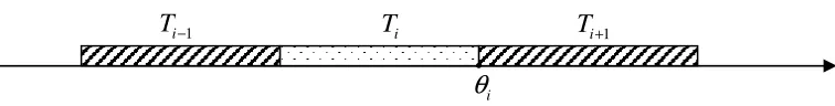
Figure 3. Bearing sets in a PVDM

Note that any two ‘consecutive’ bearing sets T ,i Ti+1 have at most one common point. Indeed,

since they are convex, their intersection has to be convex too. By assumption (2.4) this

intersection has to have zero measure. But since the support of ε is convex, it means that

1

i i

T ∩T₊ is either empty or it is a single point. In practice, either T_i is right-closed and T_i+1 is

left-closed and so T_i∩T_i+1=

{ }

θ

_i for some number θ_i∈R (cf. Figure 3) or θ_i is in only one of these sets while the other is right-open (or left-open). In any case we can define numbers

1, , n 1

θ θ ₋ as points that separate consecutive bearing sets. Let us also define θ₀ =minT₁ and

max

n Tn

θ = . Note that:

( )

( 1) ( )

i i i i

S =P T_ε =G

θ

₊ −G

θ

where Gis the cdf of ε . Hence:

1 1

0

1 1

( ) ( )

i i

i j j

j j

G

θ

G

θ

S S

− −

= =

= + = (3.9)

The convexity of support T implies that G is strictly increasing, so there exists an inverted

function G−1 and (3.9) yields:

1 1 1 i i j j G S

θ

− − = =

Consequently, with the vector S known, vector =

(

θ

₁, ,

θ

_n

)

can be unequivocally

determined. This suggests a way of defining the quality measure m_Vk. Suppose that k<n.The

definition of θ_k implies:

(

k, k, k

)

₍

k 1, k 1, k

₎

V p a θ =V p ₊ a ₊ θ

1

k

a ₊ is the solution of this equation, which is unique, because V is increasing in its second

argument. By applying the same procedure to a_k+1 and a_k+2, one can unequivocally define

2

k

a ₊ and so on. Obviously one can also define a_k−1 by considering

(

k 1, k 1, k 1

)

(

k, k, k 1

)

V p − a − θ − =V p a θ −

and, by analogy all the other elements of the quality vector left to a_k. The method of

constructing a quality measure has been demonstrated.

4. Conclusions

Random utility models are a particularly convenient way of modelling product differentiation.

In this paper we demonstrated that they can be used to examine the possibilities of creating

quality indicators. We formulated conditions sufficient for the existence of quality measures

in two broad families of RUMs: additive random utility models and pure vertical

differentiation models. In both cases, the conditions proved to be strongly related to the

convexity of the support of the model’s random component.

Our study contributes to the characteristics of RUMs: in terms of the research classification

outlined by Marley (2002), we add to the ‘characterization’ problems. Obviously there is

considerable room for improvement in our results, from the sufficient conditions for other

types of RUMs (or generalized RUMs as defined by Walker and Ben-Akiva (2002)) to a full

characterization of necessary conditions. Nevertheless, we demonstrated that the family of

demand functions for which quality measures exist is much wider than the specific functions

References

Anderson S.P, Palma A., Thisse, J.-F., 1992. Discrete Choice Theory of Product Differentiation, The MIT Press, Cambridge.

Cremer, Helmuth & Thisse, Jacques-Francois, 1991. "Location Models of Horizontal Differentiation: A Special Case of Vertical Differentiation Models," Journal of Industrial Economics, Wiley Blackwell, vol. 39(4), pages 383-90, June.

Hallak J.C., Schott, P.K , 2011. Estimating Cross-Country Differences in Product Quality, The Quarterly Journal of Economics, Vol 126, 414-474.

Khandelwal, A., 2010. The Long and Short of Quality Ladders, Review of Economic Studies 66.4, pp. 1450-1476.

Marley, A.A.J, 2002. Random utility models and their applications: recent developments, Mathematical Social Sciences, Volume 43, Issue 3, July 2002, pp. 289-302

Mussa, M., Rosen, S. 1978. Monopoly and product quality, Journal of Economic Theory, 18 (August 1978), pp. 301-317;

Shaked, A., Sutton, J., 1983. Natural Oligopolies, Econometrica, Vol. 51, No. 5, pp. 1469-1483

Suck R, 2002. Independent Random Utility Representations, Mathematical Social Sciences, Volume 43, Issue 3, July 2002, pp. 371-389.