CENTRE FOR ADVA N C E D
S PATIAL ANALYSIS
W orking Paper Series
Paper 27
Measuring Sprawl
Paul M. T
orrens
Centre for Advanced Spatial Analysis University College London
1-19 Torrington Place Gower Street
London WC1E 6BT
Tel: +44 (0) 20 7679 1782 Fax: +44 (0) 20 7813 2843
Email: [email protected] http://www.casa.ucl.ac.uk
http://www.casa.ucl.ac.uk/working_papers.htm
Date: November 2000
ISSN: 1467-1298
© Copyright CASA, UCL.
*Marina Alberti, Department of Urban Design and Planning, University of Washington. Box 355740. Seattle, WA 98195, USA.
Abstract
1.
Introduction
Suburban sprawl has several characteristics that make it, arguably, one of the most pressing concerns facing American cities (see Peiser 1989; Ewing 1994, 1997; Gordon and Richardson 1997a, b for a balanced debate about the various issues of contention surrounding the sprawl problem). Sprawl is a relatively wasteful method of urbanization, characterized by uniform low densities. It is often uncoordinated and extends along the fringes of metropolitan areas with incredible speed. Commonly, sprawl invades upon prime agricultural and resource land in the process. Land is often developed in a fragmented and piecemeal fashion, with much of the intervening space left vacant or in uses with little functionality (Ewing 1997). Sprawled areas of the city are generally over-reliant on the automobile for access to resources and community facilities. Aesthetically, these areas are often regarded as displeasing, commonly applied to urban landscapes with a blandness of design that robs vast swathes of the city of their appeal. While the character of sprawl varies across the United States, much of these characteristics (and their associated problems) share common traits. It could be argued that sprawl violates just about every premise of sustainability that a city could be judged by. Disputably, sprawl has several negative impacts on urban travel patterns. Urban sprawl also places unnecessary strains on urban service and infrastructure provision. Sprawl has been accused of encroaching on environmentally sensitive areas and is blamed for consuming resource lands and farmland. Suburban sprawl has also been attributed responsibility for pollution and ecological disturbance. Because sprawl occurs on the urban fringe and is piecemeal in its development, sites within sprawling areas tend to be located at distances from the urban core and also from each other; consequently, journeys for residents of these areas become unnecessarily long and there may be associated social and environmental consequences. In addition, it may have negative influences on urban energy efficiency, psychological and social costs to residential populations, and contribute to central city decline (see Ewing 1994, 1997).
fringes of their metropolitan expanses. Equally indicative of the magnitude of concern surrounding sprawl is the increasing attention to “Smart Growth.” In a series of initiatives, the national and local governments have begun to lay the foundation for a broad policy designed to transform the morphology of urban growth.
In academic terms sprawl is a highly contentious issue—neither its determinants nor its characteristics are fully understood. In recent years researchers have traded conceptual explorations of the sprawl phenomenon: its causes, characteristics, costs, and potential controls. Without robust empirical metrics to inform the debate, however, much of this argument remains conceptual, even speculative. The lack of understanding and consensus does little to contribute to practical, real world problem solving. On the contrary, it casts doubts upon the appropriateness and potential effectiveness of proposed policy mechanisms that are designed to counter sprawl, such as smart growth and growth management. We need robust tools that can inform the sprawl debate in a reasonable manner and serve as a foundation of consensus around which we can begin a discussion of the issues.
2.
Measuring sprawl
Theoretical debates about sprawl have generated a wealth of discussion around the issue. Recalling Ewing’s (1997) comments, however, we still lack a working definition. Sprawl is a practical, real world concern. Arguably, there is a sense of urgency attached to the sprawl problem and in many ways it is time for the theoretical debate to inform practice in more useful ways; after all, growth management legislation is sweeping through the country at paces not unlike those at which sprawl is brushing the landscape. Without a solid empirical basis for assessing the potential outcomes of what are, in many cases, quite radical legislative measures, cities are in danger of failing in their bid to control sprawl, as well as running the risk of prompting knock-on effects with unforeseen consequences. With these considerations in mind, we explore a set of methodologies that offer promise in helping us to measure sprawl. Then we consider some of the issues that must be addressed if these measures are to be put to use in practical contexts.
2.1. Measuring density
While density is almost universally regarded as one of the essential components of sprawl, the semantics of the term is hotly debated (Peiser 1989; Gordon and Richardson 1997a, b). Before we can evaluate potential techniques for quantifying sprawl densities, there are a number of important considerations in determining how the relationship between density and sprawl should be evaluated. These include the best variable to use in representing density, the density level at which a city might be regarded as sprawling, the scale at which density should be measured, and the extent of space over which density should be characterized.
sprawl as areas of the city with population densities of 0.3 to 0.5 people per acre. At these densities, they argued, parts of the city are less than adequate for efficient service provision and too high for true agricultural development (Ledermann 1967). In their work, The Costs of Sprawl (1974), the Real Estate Research Corporation (RERC) referred to low-density sprawl as a housing density of 1,360 units per square mile (quoted in Gordon & Richardson, 1997, p.99).
The scale at which density is studied is also an important consideration. Depending on the scale of observation—the metropolitan area, a district within a city, a neighborhood—measurements of urban density will look quite different. The geography over which densities should be measured is also contentious. Should an analyst use the total area of a city in her density calculation (gross density), or should she omit areas upon which people would not normally reside such as water, deserts, parks, wetlands, cemeteries, industrialized areas, disposal sites, etc. (net density) (Gordon and Richardson 1997a)? Excluded areas can, in aggregate, amount to a sizeable share of the metropolitan area. The issue becomes further complicated when we consider that the exclusion of areas such as open water and industrial areas— because of their role in influencing housing costs—might bias measurements of density (Gordon and Richardson 1997a). On the other hand, such bias is probably unavoidable and the negative and positive effects of omitted land uses may balance on the whole anyway (Zielinski 1979). In summary, we know that density is essential to sprawl, but there is little agreement about the appropriate specification of its measurement.
urban densities. If a population density gradient falls over a specified period, for example, we may say that the urban area has sprawled—in relative terms—over that time. Likewise, the gradient measure allows us to make comparisons between cities and to gauge the relative degree of sprawl between them. A city with a small population (or perhaps employment or household) density gradient can be said to be more sprawling in its relative density than a city with a comparatively larger gradient. Density gradients are not immune to the issues of specification that we have discussed, but they do have some advantageous properties that make them potentially useful for measuring sprawl.
Density gradients have the convenient property of encapsulating some key ideas in urban economics, notably input substitutions in housing (factor substitutions) and match well with theoretical ideas about the trade-off between consumer preferences regarding housing prices and costs of commuting to centers of activity (Mills and Tan 1980). Arguably, factor substitutions are influential in driving sprawl: they influence the likelihood of households to locate on the urban fringe. As we will discuss later, sprawl is a dynamic phenomenon. Because density gradients use distance from an activity center in their calculation, their evaluation is generally independent of dynamics in the structure of cities, such as shifts in the location of the urban periphery and changes in its boundary over time.
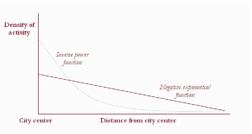
A variety of models have been developed in recent years to characterize urban densities. The main techniques for measuring density are the equilibrium function, the inverse power function, and the negative exponential function. Innovation in this area usually focuses on the parameters fitted to the distance decay component of the calculation. Equilibrium functions (Amson 1972, 1973) have been formalized in a theoretical setting, but have yet to be proven in a practical manner. Quadratic gamma functions (a classification to which the negative exponential and inverse power functions belong) have a better track record.
The mathematical structure of the inverse power function, popularized by Smeed (1963), most commonly takes on the form:
If we are to apply this formula to the measurement of sprawl, the key components here are D (the activity variable, e.g., population, households, or employment; this is expressed for a given location x , with a city center denoted as D ) and 0 α, the distance decay parameter. The value of −α is best interpreted by analyzing the first derivative of the above function. We can interpret −α as an elasticity: the ratio of the
percentage change in density dD x
D x ( ) ( )
to the percentage change in distance from an
urban center dx
x
. As you move from a city center to a periphery, density decays at
a rate of −α. In our case this represents the attenuation of density across space and allows us to compare gradients between time points, and this could offer an indication of the relative degree of sprawl in a city or between cities. The first derivative of
) (x
D can be found by:
dD x
dx x D x D
( ) ( ) = −α = −α − −α 0 1 (ii), yielding: dD x D x dx x ( ) ( )
= −α (iii)
The negative exponential function was first introduced by Bleicher (1892), but was popularized in a contemporary sense by Clark (1951). In its most general form, the function is based on the premise that population density declines monotonically (change is the same in all directions) with distance from a city center (Batty and Kwang 1992)—and this is also the case with the inverse power function—according to the equation:
D x( )= D0exp(−λx) (iv)
In the negative exponential model, −λ replaces −α ; in the last example, distance decay was formulated as an inverse power, but here it appears as a negative exponential. While essentially performing the same role, these formulations yield radically different ‘fits’ of density attenuation. Again, the value of −λ can be calculated by taking the first derivative of the above function such that:
dD x
dx D x D x
( )
exp( ) ( )
= −λ 0 −λ = −λ 0 (v),
and thus: dD x
D x dx
( )
( ) = −λ (vi)
That is, −λ, is the percentage change in density for a small change in distance from an urban center; this could be interpreted as the density gradient of sprawl.
1972)—a period in which many American cities began to suburbanize and ultimately sprawled.
Figure 1. The shape of density gradient functions (after Batty and Kwang 1992).
2.2. Surfaces of sprawl
The density gradient approach to measuring sprawl has several important advantages, as we have already seen. Nevertheless, gradients remain a linear solution to what is a two- and often three-dimensional problem. Sprawl does not occur in cross-sections and unless density gradients are calculated for many cross sections of a city, the
spatial configuration of sprawl is essentially neglected. Perhaps a better course is to
approach the problem from a two-dimensional standpoint, looking at how urban activity and the patterns of sprawl vary continuously over the entire spatial range of the city. Densities of urban attributes that are important to the sprawl problem; such as households, population, and employment; can be collected on a zonal basis (and zonal values can be assigned to a centroid point) and then converted into ‘surfaces’ of a quasi-continuous nature. There are some well-developed techniques in image processing and spatial analysis that enable these sorts of analyses to be performed. One such approach makes use of kernel density estimators.
There are a few reasons why surface smoothing may, in some cases, be desirable for the measurement of sprawl. First, spatial data for sprawl will most likely be collected in a zonal format. These data tell us that a certain level of activity has been recorded for a zone, but they tell us little about the subzonal distribution of that activity. We can infer information about individuals and single land parcels from aggregated data, but to do so runs risks of ecological fallacy. Kernel approaches allow us to make a reasoned guess at the subzonal geography of activity, based on observed activity in neighboring zones. The kernel approach also allows us to circumnavigate (or maybe ‘dodge’ is a more appropriate term) potential modifiable areal unit problems that we may encounter in measuring sprawl (see Openshaw 1983). In terms of sprawl, we may well have to work with data that aggregate entity-level activity to broad geographic zones, particularly if those data come from government sources such as the Census, or if they carry data confidentiality provisos. Also, because we are attempting to explore a multifaceted problem, we will frequently encounter data across varying scales. The surface approach can help to alleviate some of those concerns by artificially transforming data into a workable format, ‘filling-in’ the blanks that zonal geography has left, and placing data for differing zonal geographies on an even footing.
2.3. The geometry of scatter
even at the initial time of development, even when much of the land may be left vacant.
Differentiating scatter from economically efficient “discontinuous development” (Ewing 1994) can be difficult, however. The distinction involves weighing up several components of scatter: the quantity of land bypassed in the initial development wave, the length of time that land is actually withheld from development, and the ultimate use of the land (Ewing 1997). The temporal components of scatter should also be considered, as sprawl is a dynamic phenomenon—what looks like sprawling suburb today could well evolve into compact and sustainable development in later years as the pace of urban extension drives developers to fill-in previously undeveloped sites (Peiser 1989).
An examination of the geometry of scatter might be a first pass at actually measuring these characteristics so that a judgement on the presence of sprawl in a given area might be empirically based. One approach would be to use weighted centroids (Suen 1998). If the centroid of a geographic zone is the middle point of that area, then the weighted centroid is a variation that displaces the center point in the direction of concentrations of activity. We could parameterize this to reflect activities that are important to sprawl. A weighted value could be derived such that the absolute center of a zone relocates to a point where the density of a given activity is greatest. You can think of this as a ‘pulling’ of the center towards the site of greatest activity—the center point for a given area is pulled along the activity gradient in the direction of a concentration of activity. This geometric measurement may be formulated for an area of study using the following equation (Suen 1998):
(
)
S H E
H
i i i
n
= =
∑
1(vii)
where: S is the level of scatter and Hiis the number of housing units in a residential
parcel i. Eiis the Euclidean distance between the center of residential parcel i and the
( )
x w x w i i i n i i n = = =∑
∑
1 1 , and( )
y w y w i i i n i i n = = =∑
∑
1 1 (viii),where: x is the x-coordinate of the weighted areal mean of a larger grid cell; y is the y-coordinate equivalent; wiis the weight assigned to a parcel center-point i, based on
the quantity of development in that parcel; xiis the x-coordinate of a parcel center-point i; and yiis the y-coordinate equivalent for a parcel center-point i.
The calculation of a weighted mean starts with parcels of development occupying a larger grid tile. Once the absolute center-points of the tile have been identified, the
weighted center of the tile cell is calculated. The tile’s center is shifted according to
Figure 2. Diagram illustrating the relative positioning of parcel center-points, the weighting of parcels by units of development, unweighted tile centers, and weighted
tile centers for a hypothetical area of study (adapted from Suen 1998).
Figure 3. Diagram illustrating two cases of scatteration (adapted from Suen 1998).
2.4. Fractal dimensions of sprawl
that are useful for describing cities, see Batty and Longley (1994)). If we consider the traditional integer dimensions of an urban area, we might imagine a city with a dimension of zero (a city existing on a point). A city with a dimension of one (a city existing as a line) might correspond to something like Soria Y Mata’s ‘La Cuidad Lineal’ or Frank Lloyd Wright’s ‘Mile-High Skyscraper City’. A city with a dimension of two (one that fully occupies a two-dimensional plane) might also be conceived of, such as Wright’s ‘Broadacre City’. Indeed, we might imagine a city that fully occupies three dimensions, such as Dantzig and Saaty’s ‘Compact City’ (Batty and Longley 1997). While the existence of one-, two-, and three-dimensional cities might easily be conceptualized in a theoretical context, in a practical setting such forms are unlikely to exist; cities are not that orderly! Most cities do not occupy a single or multiple-dimensions fully; their dimensionality does not fit neatly into whole number classifications. On the contrary, cities are more ‘fuzzy’; their dimensions usually form real numbers, occupying fractions of a dimension.
Fractals hold much promise as an indicator of the level of scattering in urban development and thus as a measure of sprawl-like leapfrogging. Sprawl is about space
filling (or at least an inefficiency or an unsustainability in space filling). Fractals offer
ways in which we can measure the extent to which phenomena such as sprawl manifest themselves at levels between dimensions. Sprawl lies somewhere between well-developed compact built environments and the countryside, which for the most part lacks any urban development per se (Figure 4). Also, like fractals, sprawl is self-similar in its spatial pattern (Figure 5). Scatter is evident at an urban scale, intra-urban scale, and also at the neighborhood level. Fractals are a powerful tool for capturing those properties. In its most general form, a fractal dimension may be calculated as:
F l
a
ij ij
= 2 ln
ln (ix),
closer the value of the fractal dimension approximates two, the more compact— perhaps even sustainable—the development contained within the space may be considered. As the fractal dimension nears one, development becomes less compact and may be understood to be scattered and sprawl-like. Also, we can associate certain morphologies of development, such as sprawl, with specific signatures; these signatures can be calculated as fractals. For example, Mesev, Longley, Batty et al. (1995) have calculated signatures for density using fractal-based power functions.
Figure 5. A fractal from the Mandlebrot Set, demonstrating self-similarity (source:
author).
2.5.Measuring the built environment of sprawl
The aesthetic characteristics of sprawl—images that it conjures in the mind’s eye— are one of the less tangible qualities of the phenomenon, yet they are also amongst its key components. Sprawl is as much an aesthetic architectural and design-based problem as it is an issue of urban structure. Urban sprawl is widely regarded as a lazy and undisciplined expression of urbanization (Gordon and Richardson 1997a), almost universally met with criticism and distaste: “Urban sprawl, roller-painted across the countryside is often without form, grace, or a sense of community. Planning philosophies aimed to strike down this amorphous creature should only gladden our hearts” (Lessinger 1962, p.159). The aesthetic qualities of sprawl certainly provoke a level of eloquence in commentary, but the subjective nature of aesthetic sensitivities leave us with little room for quantification.
scatter, although it is radial rather than planar in form. Ribbon sprawl generally manifests itself as strips of commercial development (normally retail outlets and related premises) that flank the sides of highways and main thoroughfares. Exit-parisitic retail development is an associated component: the clustering of retail establishments (hotels, gas stations, fast food restaurants, etc.) close to highway exit ramps (see Torrens 1998). Ribbon sprawl is composed of segments of developed land that are compact in themselves but which extend axially and leave the intervening space undeveloped (Harvey and Clark 1965). This creates walls of commercial development (often buffered by large ‘seas’ of car parking) that restrict access to much of the space around them.
Because the aesthetic concerns about sprawl are almost all design-based, we need to examine the built environment of sprawl to measure its aesthetic qualities. Ideally, to do this we would (and probably should) interview a representative sample of residents and generalize our findings on aesthetics to the urban population as a whole. However, such surveys would undoubtedly be both costly and time consuming. Alternatively, we could follow in the tradition of automated analyses of built environments (Ward, Phinn and Murray 2000 is one such recent work) and devise an automated approach to measuring aesthetics. The idea here would be to derive a “mathematical characterisation of urban patterns” (Webster 1995). There are two main routes that can be taken. Both rely on digital imagery of urban environments, usually aerial photographs or scenes captured from remote sensing platforms.
Architectural techniques relate images to known primitives—or marker points—for
the built environment. Photogrammetric techniques associate the spectral signature of an image with typologies and characteristics of urban land covers or uses.
such primitives are useful in characterizing urban built form (see Steadman, Bruhns and Gakovic 2000). With reference to the interests of this paper, we may be able to discern key primitives associated with sprawl: architectural configurations, the spatial structure of phenomena such as ribbon sprawl, lot configurations, or arrangements of buildings and land parcels on the urban fringe; and perhaps we could relate these to digital imagery for automated analysis and measurement.
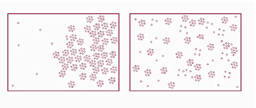
The photogrammetric approach is a little less straightforward, simply because there are a wide variety of techniques that we might employ. Broadly speaking, there are two main approaches, both based on pattern recognition in the digital image: techniques that deal with raw imagery and methods that are applied on transformed images (Webster 1995). Amongst the techniques that deal with raw images, perhaps the most basic approach would be to look at the standard deviation of individual pixels from average values (reflectance, corresponding to the albedo value of a given urban surface, for example) for the entire scene (Webster 1995).
Mathematically, this standard deviation can be calculated using the following equation:
(
)
2 12 1
∑
= −
= n
i
i X
X N
σ (x)
The standard deviation (σ2
) of individual pixels from the average value of the entire scene is a summation of the difference between the values of individual pixels (X )i
values, despite being radically different in their spatial structure and their inference of sprawl. Nevertheless, the statistic may be a useful starting point for building relatively more solid measurements of the built environment of sprawl.
Figure 6. Two images of differing spatial character yield similar standard deviation values.
Proceeding from this approach, it is possible to generate a number of measures of the condition of an urban landscape: entropy (the ‘sameness’ of built form), homogeneity in pixel value, and relative contrast value for urban features (a proxy for building materials) (see Webster 1995 for details).
2.6. Ecology of sprawl
In many cases, sprawl can have a profound influence upon ecological systems. It can interfere with habitats by fragmenting faunal and floral habitat ranges and deforestation can destroy habitats altogether. Urbanization, particularly sprawl can have negative influences on hydrological systems, principally by reducing the permeability of land and increasing surface runoff, with implications for the introduction of pollutants into ecosystems (Ewing 1994). There are a number of metrics that we can use to quantify these effects, particularly their spatial distribution. Many of the metrics also serve as good indices of other sprawl characteristics outside of ecology.
We can measure the effect of urban sprawl on ecology by looking at its effects on the composition and spatial distribution of habitat patches. Several ecological studies have demonstrated that the ecological conditions of any patch are related to ecological pattern at the landscape scale (Turner 1989; McDonnell, Pickett, Groffman et al. 1997). Numerous metrics in landscape ecology have been developed to quantify such pattern and its effects on disturbance regimes (O'Neill, Krummel, Gardner et al. 1988; Turner 1989; Li and Reynolds 1994; McGarigal and Marks 1995; Gustafson 1998). Based on an empirical study recently conducted by Alberti and Botsford (2000) in the Puget Sound area, we propose a set of metrics to quantify characteristics of sprawl that we hypothesize are relevant to ecological conditions. Many of these metrics can be extended to measure other characteristics of sprawl.
Metrics of landscape patterns aim to measure two major characteristics of the landscape: its composition and its spatial configuration (Turner 1989). Landscape
composition refers to the presence and amount of different patch types within the
landscape, without explicitly describing its spatial features. Two common metrics of landscape composition are the Shannon Diversity Index, which measures the degree of diversity in a given landscape and the Shannon Evenness Index, which measures the distribution of area among patch types. Landscape configuration refers to the spatial distribution of patches within the landscape. Examples of configuration metrics are patch size, edge-to-interior-ratio, nearest-neighbor, fractal dimension, and contagion. In landscape ecology these metrics are good predictors of the ecosystem's ability to support important ecosystem functions (Turner and Gardner 1991). Ecological studies have shown, for example, that patch size is positively correlated to species and habitat diversity. Edge-to-interior ratio and nearest-neighbor probabilities reflect the degree of landscape fragmentation. Fractal dimension reflects the extent of human impacts. Contagion is an important measure of contiguous habitat types (O'Neill, Krummel, Gardner et al. 1988; Turner and Gardner 1991).
These metrics allow us to measure the pattern and configuration of ecological disturbances in the natural and built environments caused by sprawl; additionally urban sprawl patterns—and important characteristics such as scatter, fragmentation, homegeneity, connectivity, etc.—can be quantified using a variety of these metrics (Alberti 2001). However as Webster (1995) points out “the choice of the metrics in measuring patterns should aim to achieve the best discrimination between categories within a particular category scheme used to describe a specific phenomenon.” For example, different pattern metrics of urban sprawl will best discriminate building density, development scatter, and habitat fragmentation. Furthermore, the choice of scale at which the metric is measured, both the resolution and the geographic extent will be relevant to the ability of a metric to represent these phenomena (Webster 1995).
evenness across the classes, the level of aggregation of each class into patches, the frequency distribution of patch size, and the spatial distribution of these patches in the landscape. A careful interpretation of spatial metrics is possible when the ability of each measure to quantify a single component of pattern is fully understood.
Sprawl results in greater landscape heterogeneity and fragmentation (compared with more compact forms of development). Several patch metrics can be applied to measure these patterns on an urban to rural gradient. The number of patches of a specific land use and land cover type is a useful index of the urban landscape heterogeneity (sameness of design and use). In addition patch density provides a measure of landscape structure that can facilitate comparisons among landscapes of varying size. Patch density in the entire landscape mosaic could serve as a good heterogeneity index. Measured as the number of patches on a per-unit-area basis for a particular patch type, patch density could serve also as a good fragmentation index (perhaps a proxy for scatter). Similarly Mean Patch Size (MPS) can serve as a fragmentation index:
) 10000
1 (
1
i n
j ij
n a MPS
∑
=
= (xi)
MPS equals the sum of the areas of all patches of the corresponding patch type, divided by the number of patches of the same type, divided by 10,000 (to convert to hectares) (McGarigal and Marks 1995). A landscape with a smaller mean patch size for the target patch type than another landscape might be considered more fragmented. Similarly, within a single landscape, a patch type with a smaller mean patch size might be considered more fragmented. Variability in patch size can be measured with Patch Size Standard Deviation.
the Contagion index was designed to measure habitat characteristics, it can readily be applied to quantify urban phenomena by measuring parcels or patches of land with associated land use in lieu of patches. The common specification of a Contagion index takes the form (Li and Reynolds 1994):
( )
( )
( )
100ln 2 ln 1 1 1 1 1 ∗ − + =
∑∑
∑
∑
= = = = m g g P g g P C m i m j m j ij ij i m j ij ij i (xii),where: C is the contagion, P is the proportional abundance of category type i, i g isij
the number of adjacencies between cells of category type i and all other category types, and m is the total number of category types. Contagion is based on cell adjacencies as opposed to patch adjacencies. It measures both patch dispersion and interspersion. Landscapes consisting of large patches of similar land cover or land use category have a greater number of adjacent cells. Where contagion is low, urban areas can be said to be comprised of many small and dispersed patches of various land cover or land uses categories (they are fragmented or ‘leapfrogged’). However, Contagion indices do not offer any indication of the degree of connectivity between patches or land use and in this respect they may fall short as indicator of the urban structure. Furthermore since Contagion is related to pixel aggregation both patch size and shape influence this measure. Simpler patch configurations and larger patch sizes result in higher Contagion values for landscapes of the same composition.
(
)
[
]
(
)
1001 ln ln 2 1 1 1 ⋅ − − − =
∑
=∑
−+ m m E e E e IJI m i k ik ik m i (xiii)It can be applied to the landscape and class level. When applied to land use it measures the degree of interspersion of land uses. Contrary to Contagion, this index measures patch adjacencies, not cell adjacencies and can be more appropriate in representing the urban structure. However the interspersion index only measures interspersion and it is not affected by the size, contiguity, or dispersion of patches; thus it captures only one aspect of sprawl.
Another important aspect of sprawl is the proximity of land uses, as this has important implications for landscape homogeneity (sameness of design; homogeneity), land-use mixing, and accessibility. Again, we can use some techniques from landscape ecology to measure these characteristics. The landscape metric, Proximity, can be calculated as the sum of patch area divided by the nearest edge-to-edge distance squared between the patch and the corresponding patch type within a specified radius (McGarigal and Marks 1995):
∑
= = n s ijs ijs h a PROXIM 12 (xiv)
The proximity metric could be modified to estimate the proximity of two different patch types within a specified radius. The Mean Proximity Index (MPI) for patches within a specified class measures the degree of isolation and fragmentation of the corresponding patch type (perhaps a substitute for accessibility) but it is difficult to interpret when patches occur in high density or span the entire landscape (Gustafson 1998).
able to distinguish overall landscape pattern caused by a unique spatial distribution of patches. Each of the measures presented here quantifies an important component of the landscape that needs to be considered in monitoring sprawl.
These metrics offer much promise as practical tools for quantifying the spatial heterogeneity of the urban landscape and help gauge the ecological effects of urban sprawl. Their operationalization is relatively straightforward. Identifying and quantifying patches of activity or use can be done with the parcel-level geographic information system databases now available in many metropolitan areas. A cursory approach would be to use spatial analysis techniques to rasterize a cityscape into a tessellation of grid cells based on an attribute or attributes of the landscape. That tessellation can then be filtered such that the cells that comprise it are generalized and smoothed recursively, yielding aggregated patches of cohesive activity. A suite of spatial analysis techniques are also available that will enable analysts to classify a layer of a geographic information system by attribute and dissolve polygon boundaries, leaving behind cohesive spatial units—patches—of activity. Several software packages (e.g., Fragstats, Path Analyst and the Geographic Resource Analysis Support System (GRASS)) are also available to evaluate these metrics on large data sets.
2.7. Accessibility
tracts) in sprawling areas; for the generic low-density residential landscape everything is dispersed, making all trips longer. Looking at the issue of accessibility from the perspective of a metropolitan area, it is also worth noting that sprawl, as a fringe phenomenon, situates areas of the city at great distance from central cities, and distances residents from the resources they offer (central transport stations and cultural amenities, for example).
The traditional methods by which accessibility might be quantified derive from transportation, economics, and regional science and may be summarized into three broad groups: cumulative opportunities measures, gravity-based measures, and utility-based measures (Handy and Niemeier 1997). Cumulative opportunities measures generally count the number of opportunities that can be visited within a given travel time. These measures therefore provide an indication of the volume of potential destinations or activities available to trip-makers in a given area, rather than distance to those opportunities (Handy and Niemeier 1997).
Gravity-based measures follow in the tradition of the spatial interaction model (see Torrens (2000)). A spatial interaction model is generally employed to predict the size and direction of spatial flows using independent variables that measure some structural properties of the area in question. In the context of measuring accessibility as an indicator of sprawl, the spatial pattern of trips could be calculated using structural variables such as the distribution of workers’ homes, the distribution of employment locations, and the costs—in monetary terms, or perhaps in units of traveling time—of navigating the city.
Essentially, the gravity formula is conceptually based on ideas from Newtonian physics. The gravity model scheme is not at all unlike the idea of satellites orbiting around a central center of gravity, which influences the gravitational pull on each satellite with a force proportional to the mass of bodies in the system. The gravity accessibility calculation is premised on the idea that the accessibility (trip) between an origin and a destination (Aij) is the summation of several components: the capacity of an origin to generate trips (Wi ), the ability of activities at a destination to attract those trips (Wj ), the distance over which the trips must be traversed ( )
α
ij
normalizes the calculation to take account of the fact that (Wi ) and (Wj ) are not expressed in units of flow (Thomas and Huggett 1980). Mathematically, this can be expressed as:
∑
= ⋅ = n j ij j i ij d w w k A 1 α (xv)Utility-based measures of accessibility derive from spatial choice models and decision theory. They have the advantage of being more behaviorally rooted than gravity models. Broadly speaking, utility measures determine the utility of adopting one decision from a set of available choices. In terms of accessibility, a utility measure can be devised that weighs up the utility value of trip choices available within a given distance from a location. We can use the utility value as a proxy for accessibility. Areas of a city with large utility values for transportation may be considered to be more accessible, in relative terms, than areas with comparatively low utility values. The more accessible an area is, the greater the likelihood that the development is compact and sustainable. As accessibility wavers, we may suggest that an area has sprawled.
Mathematically, utility-based measures are commonly calculated as logit models. In our case, accessibility may be calculated as the denominator of a multinomial logit model such that:
( )
=∑
∈ ∀ n C C n n n VA ln exp ( ) (after Handy and Niemeier (1997)) (xvi)
In the above equation, Anis the accessibility measure for an individual (or perhaps a
household), n and Cn is the available choice set of opportunities that can be visited
example, travel time and distance) (Handy and Niemeier 1997). The logsum, ln
∑
, indicates the desirability of the full choice set C . We can include variables that represent the attributes of available transport choices in the city to expand the utility calculation: the attractiveness of the destination, any barriers that might delay trips (such as fragmented development), and the socioeconomic characteristics of the individual or household making the trip (reflecting individual tastes and preferences). Of course, utilities that cannot be expressed in distance or financial terms are notoriously difficult to measure (see Torrens 2000).Isochronic accessibility measures (also known as cumulative opportunities measures) deal with accessibility in terms of the amount of time it takes to reach a given location from any place within a city (see Lee and Goulias 1997; O'Sullivan 2000). They perform the same functions, in terms of measuring sprawl, as our other measures: they give us an idea of the relative dispersal of opportunities in a city. In this case, however, impedence is measured in terms of time, rather than distance (in a Euclidean or weighted sense). They answer questions of the form: given a time budget of X hours, how far can I get in the city? They may be expressed, for example, in the following form:
∑
= = 1,0
10.5
n n i
n R
A (xvii)
Where A is the isochronic accessibility of an origin zone i, i R is the number ofn
destinations that can be reached within the nth annulus (i.e., in this example, between 0.5n km and 0.5*(n–1 km) from the origin zone i), and 0.5n represents a 5 km opportunity.
limits are also proposed in calibrating these accessibility measures: the choice of a cut-off point or value for travel distance or time, representation of the travel impedance function, and whether to use revealed (actual) or preferred (ideal) behavior in calibrating utility-based measures.
However, these measures do show a great deal of promise in calculating the relative accessibility of destinations for different areas of the city. In this way, the relative level of residential accessibility (as defined by Ewing) might be measured. Equally, the level of accessibility between homes could be calculated by any of the above measures, serving as an indicator of destination accessibility. Both of these characteristics can give us an empirical idea of the relative degree of compactness and sprawl in a city, with inferences to scatter, spatial structure, and density of activity.
3.
Issues of concern
We have discussed several potential measurements for quantifying suburban sprawl. Each of these measurements has advantages for capturing unique characteristics of sprawl (or even several such characteristics): density, scatter, the built environment, ecology, and accessibility. However, there are a number of important concerns that must be considered in applying these metrics to the evaluation of sprawl, including data availability, dynamics, pattern and process, scale, and agency.
3.1. Data
3.2. Sprawl as a dynamic phenomenon
It is notable that sprawl is commonly treated as a static phenomenon. This is a misconception; sprawling areas of the city are at the forefront of dynamic urban growth. By misinterpreting sprawl as static, planners and policy-makers risk making incorrect judgements, and researchers are neglecting elementary components of the problem. It is important that measures of sprawl recognize and treat the phenomenon as a dynamic.
“The sprawl of the 1950s is frequently the greatly admired compact urban area of the early 1960’s. An important question on sprawl maybe, “How long is required for compaction?” as opposed to whether or not compaction occurs at all…The concept of time span is important in the identification and measurement of sprawl. The application of static measures to dynamic areas can easily result in the misidentification of an area as sprawl when it is really a viable, expanding, compacting portion of the city” (Harvey and Clark 1965, p.6).
Part of the problem is that many of the measurements we have proposed are themselves static—they capture properties of sprawl in a snapshot of time. In order to examine sprawl in a truly dynamic fashion it may be necessary to employ a simulation model. These metrics could still be used, to calibrate the model against observed conditions in the real world. The essential dynamics of the problem would be captured in the simulation though. With this in mind, there are a number of approaches that might be followed.
dynamics inherent in land use and land cover change by combining a microsimulation of actor choices (location, housing, travel, production consumption and land development) and a Monte Carlo simulation of the land cover change on a 30 meter grid cell structure (Waddell and Alberti 2000). This represents one possible approach to capturing the dynamics of the sprawl problem.
The challenge in modeling sprawl dynamics stems from the fact that metropolitan areas exhibit some fundamental features of complex and self-organizing systems. Cellular automata (CA) models have been used successfully to simulate a wide range of environmental systems including fire spread and forest dynamic (Green 1989, 1994) as well as urban systems simulation (White 1998; O'Sullivan and Torrens 2000). Additionally, more recent development of multi-agent systems (Minar, Burkhart, Langton et al. 1996; Batty, Jiang and Thurstain-Goodwin 1998; Terna 1998; Batty 1999; Batty and Jiang 1999; Schelhorn, O'Sullivan, Haklay et al. 1999) and agent-based CA (Portugali, Benenson and Omer 1997; Portugali 2000) provide a useful framework for modeling the aggregate effects that results from numerous locally made decisions of many intelligent and adaptive agents in an interactive and dynamically adaptive environment.
3.3. Pattern versus process
3.4. Scale-dependency and sensitivity
Perhaps the choice of measurement scale is one of the most critical issues in defining appropriate indices for measuring sprawl. The choice ultimately depends upon the relevant scale at which the hypothesized socio-economic and biophysical processes that drive or are affected by sprawl operate. However the sensitivity of spatial metrics to scale should be considered before applying any spatial statistics. None of the metrics that we have discussed here (save perhaps fractal dimension) are scale-independent. There is a vast literature that examines the effect of scale both in terms of resolution and geographic extent on pattern analysis (Turner 1990). Most landscape metrics are scale dependent and are relevant to processes operating only at specific spatial scales (O'Neill 1988). Since almost all the metrics proposed here to measure sprawl are affected by scale an exploratory pattern analysis of the landscape would be critical to detect the range of scales over which spatial metrics are relatively insensitive to pixel size or spatial extent. Within the range detected the metrics value will then depend on the actual pattern and provide a useful measure for comparison across landscapes and scales. Rather than allowing scale-sensitivity to foreshadow any attempt to measure sprawl, this is simply a matter of learning to live with the inadequacies of the tools and being aware of their limitations.
3.5. Weaving agency into the equation
these models, however, both conceptual and technical. Importantly, it is unsure how best to represent institutions such as planning regimes, businesses, and the government in multi-agent systems. The agent-based simulation approach is notoriously biased towards individualism (O'Sullivan and Haklay 2000). Equally, the question of designing agents that fulfill multiple roles—head of household, employee, neighborhood activist—is a tricky one. Nevertheless, the potential for exploring the causes and manifestations of sprawl with these simulations is rich.
4.
Conclusions
We have reviewed several techniques for evaluating suburban sprawl in an empirical manner. Sprawl is a multifaceted problem with several related characteristics that we can attempt to measure: density, scatter, the built environment, and accessibility. We have proposed a set of metrics for quantifying these attributes, including density gradients, surface-based approaches, geometrical techniques, fractal dimension, architectural and photogrammetric techniques, measurements of landscape composition and spatial configuration, and accessibility calculations.
5.
References
Alberti, M. (2001). Quantifying the Urban Gradient: Linking Urban Planning and Ecology. In Avian Ecology in an Urbanizing World. J. M. Marzluff, R. Bowman, R. McGowan and R. Donnelly. New York, Kluwer.
Alberti, M. and E. Botsford (2000). Behavior of land use and land cover metrics along an urban-rural gradient. Working Paper, Urban Ecology Research Laboratory, Department of Urban Design and Planning, University of Washington. Seattle.
Alperovich, G. and J. Deutsch (1992). 'Population density gradients and urbanisation measurement'. Urban Studies 29(8): 1323-1328.
Amson, J. C. (1972). 'Equilibrium models of cities 1. An axiomatic theory'.
Environment and Planning 4: 429-444.
Amson, J. C. (1973). 'Equilibrium models of cities 2. Single-species cities'.
Environment and Planning 5: 295-338.
Batty, M. (1999). Multi-agent approaches to urban development dynamics. Research proposal for the Environmental and Social Research Council. Centre for Advanced Spatial Analysis, University College London. London.
Batty, M. and B. Jiang. (1999). Multi-Agent Simulation: New Approaches to Exploring Space-Time Dynamics Within GIS. CASA Working Paper 10. Centre for Advanced Spatial Analysis (CASA), University College London. London. http://www.casa.ucl.ac.uk/working_papers.htm
Spatial Analysis (CASA), University College London. London. http://www.casa.ucl.ac.uk/working_papers.htm
Batty, M. and S. K. Kwang (1992). 'Form follows function: reformulating urban population density functions'. Urban Studies 29(7): 1043-1070.
Batty, M. and P. Longley (1994). Fractal Cities. London, Academic Press.
Batty, M. and P. Longley (1997). 'The fractal city'. Architectural Design 67(9/10): 74-83.
Bleicher, N. (1892). Statistiche Beschreibung der Stadt Franfurt-am-Main und ihrer Bevölkerung. Frankfurt-am-Main.
Bussière, R. (1968). The spatial distribution of urban populations. International Federation for Housing and Planning and Le Centre de Recherche d'Urbanisme. The Hague and Paris.
Clark, C. (1951). 'Urban population densities'. Journal of the Royal Statistical Society,
Series A 114: 490-496.
Ewing, R. (1994). 'Causes, characteristics, and effects of sprawl: a literature review'.
Environmental and Urban Issues 21(2): 1-15.
Ewing, R. (1997). 'Is Los Angeles-style sprawl desirable?'. Journal of the American
Gordon, P. and H. W. Richardson (1997a). 'Are compact cities a desirable planning goal?'. Journal of the American Planning Association 63(1): 95-106.
Gordon, P. and H. W. Richardson (1997b). 'Where's the sprawl?'. Journal of the
American Planning Association 63(2): 275-278.
Green, D. G. (1989). 'Simulated effects of fire, dispersal and spatial pattern on competition within vegetation mosaics'. Vegetation 82: 139-153.
Green, D. G. (1994). 'Connectivity and complexity in ecological systems'. Pacific
Conservation Bilogy 1(3): 194-200.
Gustafson, E. J. (1998). 'Quantifying landscape spatial pattern: what is the state of the art?'. Ecosystems 1: 143-156.
Handy, S. L. and D. A. Niemeier (1997). 'Measuring accessibility: an exploration of issues and alternatives'. Environment and Planning A 29: 1175-1194.
Harvey, R. O. and W. A. V. Clark (1965). 'The nature and econmics of sprawl'. Land
Economics 61(1): 1-9.
Ledermann, R. C. (1967). The city as a place to live in. In Metropolis on the Move:
Geographers Look at Urban Sprawl. J. Gottmann and R. A. Harper. New York,
John Wiley & Sons.
Lessinger, J. (1962). 'The cause for scatteration: some reflections on the National Capitol Region Plan for the Year 2000'. Journal of the American Institute of
Planners 28(3): 159-170.
Li, H. and J. F. Reynolds (1994). 'A simulation experiment to quantify spatial heterogeneity in categorical maps'. Ecology 75: 2446-2455.
McDonnell, M., S. Pickett, P. Groffman, P. Bohlen, R. Pouyat, W. Zipperer, R. Parmelee, M. Carreiro and K. Medley (1997). 'Ecosystem processes along an urban-to-rural gradient'. Urban Ecosystems 1: 21-36.
McGarigal, K. and B. Marks. (1995). FRAGSTATS: Spatial Pattern Analysis Program for Quantifying Landscape Structure. General Technical Report PNW-GTR-351. USDA Forest Service.
Mesev, T. V., P. A. Longley, M. Batty and X. Yichun (1995). 'Morphology from imagery: detecting and measuring the density of urban land use'. Environment and
Planning A 27(5): 759-780.
Mills, E. S. (1972). Studies in the Structure of the Urban Economy. Johns Hopkins Press for Resources for the Future. Baltimore.
Mills, E. S. and J. P. Tan (1980). 'A comparison of urban population density functions in developed and developing countries'. Urban Studies 17: 313-321.
Muth, R. (1969). Cities and Housing. Chicago, University of Chicago Press.
O'Neill, R. V., J. R. Krummel, R. H. Gardner, G. Sugihara, B. Jackson, D. L. DeAngelis, B. T. Milne, M. G. Turner, B. Zygmunt, S. W. Christensen, V. H. Dale and R. L. Graham (1988). 'Indices of landscape pattern'. Landscape Ecology 1: 153-162.
Openshaw, S. (1983). The Modifiable Areal Unit Problem. Norwich, GeoBooks.
O'Sullivan, D. (2000). 'Using desktop GIS for the investigation of accessibility by public transport: an isochrone approach'. International Journal of Information
Science 14(1): 85-104.
O'Sullivan, D. and M. Haklay (2000). 'Agent-based models and individualism: is the world agent-based?'. Environment and Planning A 32(8): 1409-1425.
O'Sullivan, D. and P. M. Torrens (2000). Cellular models of urban systems. In
Theoretical and Practical Issues on Cellular Automata. S. Bandini and T.
Worsch. London, Springer-Verlag.
Peiser, R. (1989). 'Density and urban sprawl'. Land Economics 65(3): 193-204.
Portugali, J. (2000). Self-Organization and the City. Berlin, Springer-Verlag.
Schelhorn, T., D. O'Sullivan, M. Haklay and M. Thurstain-Goodwin. (1999). STREETS: an agent-based pedestrian model. CASA Working Paper 9. University College London, Centre for Advanced Spatial Analysis. London.
Sipper, M. (1997). Evolution of Parallel Cellular Machines: The Cellular
Programming Approach. Berlin, Springer.
Smeed, R. J. (1963). 'The effect of some kids of routeing systems on the amount of traffic in the central areas of towns'. Journal of the Institution of Highway
Engineers 10(1): 5-26.
Steadman, P., H. R. Bruhns and B. Gakovic (2000). 'Inferences about built form, construction, and fabric in the nondomestic building stock of England and Wales'.
Environment and Planning B 27(5): 733-758.
Steadman, P., H. R. Bruhns, S. Holtier, B. Gakovic, P. A. Rickaby and F. E. Brown (2000). 'A classification of built forms'. Environment and Planning B 27: 51-72.
Suen, I.-S. (1998) Measuring Sprawl: A Quantitative Study of Residential Development Pattern in King County, Washington. Ph.D. Thesis. University of Washington, Seattle.
Terna, P. (1998). 'Simulation tools for social scientists: Building agent based models with SWARM'. Journal of Artificial Societies and Social Simulation 1(2). http://www.soc.surrey.ac.uk.JASSS/1/2/4.html.
Thomas, R. M. and R. J. Huggett (1980). Modelling in Geography: A Mathematical
Torrens, P. M. (1998) Everything Must Go! The Geography of Retail Change in America's Northeastern Megalopolis, 1977 to 1992. Master's Thesis. Indiana University, Bloomington.
Torrens, P. M. (2000). How Land-Use-Transportation Models Work. CASA Working Paper 20. Centre for Advanced Spatial Analysis, University College London. London. http://www.casa.ucl.ac.uk/working_papers.htm
Turner, M. G. (1989). 'Landscape ecology: The effect of pattern on process'. Annual
Review of Ecological Systems 20: 171-197.
Turner, M. G. and R. H. Gardner, Eds. (1991). Quantitative Methods in Landscape
Ecology. Ecological Studies. New York, Springer.
Waddell, P. and M. Alberti (2000). Integrated simulation of real estate development
and land cover change. Fourth International Conference on Integrating GIS and
Environmental Modeling (GIS/EM4), Banff, Alberta, Canada.
Ward, D., S. R. Phinn and A. T. Murray (2000). 'Monitoring growth in rapidly urbanizing areas using remotely sensed data'. The Professional Geographer 52(3).
Webster, C. J. (1995). 'Urban morphological fingerprints'. Environment and Planning
B 22: 279-297.
White, R. (1998). 'Cities and cellular automata'. Discrete Dynamics in Nature and
Society 2: 111-125.