I n e r ti al s e n s o r-b a s e d k n e e
fl exio n/ e x t e n si o n a n g l e
e s ti m a ti o n
C o o p er, G, S h e r e t , I, M c Milli a n , L, Siliv e r di s, K, S h a , N, H o d gi n s ,
D, Ke n n ey, LPJ a n d H o w a r d , D
h t t p :// dx. d oi.o r g / 1 0 . 1 0 1 6 /j.j bio m e c h . 2 0 0 9 . 0 8 . 0 0 4
T i t l e I n e r ti al s e n s o r-b a s e d k n e e fl exio n/ ex t e n si o n a n g l e e s ti m a tio n
A u t h o r s C o o p er, G, S h e r e t , I, M c M illi a n , L, Siliv e r di s, K, S h a , N, H o d g i n s , D, Ke n n ey, LPJ a n d H o w a r d , D
Typ e Ar ticl e
U RL T hi s v e r si o n is a v ail a bl e a t :
h t t p :// u sir. s alfo r d . a c . u k /i d/ e p ri n t/ 1 2 6 2 8 / P u b l i s h e d D a t e 2 0 0 9
U S IR is a d i gi t al c oll e c ti o n of t h e r e s e a r c h o u t p u t of t h e U n iv e r si ty of S alfo r d . W h e r e c o p y ri g h t p e r m i t s , f ull t e x t m a t e r i al h el d i n t h e r e p o si t o r y is m a d e f r e ely a v ail a bl e o nli n e a n d c a n b e r e a d , d o w nl o a d e d a n d c o pi e d fo r n o
n-c o m m e r n-ci al p r iv a t e s t u d y o r r e s e a r n-c h p u r p o s e s . Pl e a s e n-c h e n-c k t h e m a n u s n-c ri p t fo r a n y f u r t h e r c o p y ri g h t r e s t r i c ti o n s .
Title: Inertial sensor-based knee flexion/extension angle estimation
Authors: Glen Cooper1, Ian Sheret2, Louise McMillian2,
Konstantinos Siliverdis2, Ning Sha1, Diana Hodgins3,
Laurence Kenney1, David Howard1
1
Centre for Rehabilitation and Human Performance Research,
University of Salford, UK
2
Analyticon, Tessella Support Services Plc, Stevenage, UK
3
European Technology for Business Ltd, Codicote, UK
Submission Type: Original Article
Corresponding Author: Glen Cooper
Address: Centre for Rehabilitation & Human Performance
Research,
Brian Blatchford Building,Frederick Road Campus,
University of Salford, Salford, UK. M6 6PU
Telephone Number: +44 (0)161 2952249
Fax Number: +44 (0)161 2952668
Email Address: [email protected]
Key Words: Kalman Filters, Joint Angles, Inertial Measurement Unit,
Accelerometers.
Abstract
A new method for estimating knee joint flexion/extension angles from segment
acceleration and angular velocity data is described. The approach uses a
combination of Kalman filters and biomechanical constraints based on
anatomical knowledge. In contrast to many recently published methods, the
proposed approach does not make use of the earth’s magnetic field and
hence is insensitive to the complex field distortions commonly found in
modern buildings. The method was validated experimentally by calculating
knee angle from measurements taken from two IMUs placed on adjacent
body segments. In contrast to many previous studies which have validated
their approach during relatively slow activities or over short durations, the
performance of the algorithm was evaluated during both walking and running
over 5 minute periods. Seven healthy subjects were tested at various speeds
from 1 to 5 miles/hour. Errors were estimated by comparing the results
against data obtained simultaneously from a 10 camera motion tracking
system (Qualysis). The average measurement error ranged from 0.7 degrees
for slow walking (1 mph) to 3.4 degrees for running (5mph). The joint
constraint used in the IMU analysis was derived from the Qualysis data.
Limitations of the method, its clinical application and its possible extension are
1. Introduction
The use of lightweight, low power, MEMS inertial sensors to measure acceleration or angular velocity is now widespread in the clinical community. Inertial sensor data have been used to infer: activity type/intensity; falls and falls risk; muscle activity; and gait events [1-3]. However, accelerometers together with rate gyroscopes can also be used to estimate orientation relative to an inertial frame. While high accuracy estimation of inclination is possible [4], such an approach is limited by the lack of absolute orientation information in the horizontal plane (azimuth). Relative orientation estimation is possible by integration of gyro signals in this plane, but such an approach is susceptible to drift. Consequently, techniques that take advantage of the earth’s magnetic field, that provides information on azimuth, are often adopted. Commercial systems that adopt such an approach are now widely available (e.g.
www.xsens.nl). However, despite attempts to deal with the heterogeneity of the earth’s magnetic field inside modern buildings [5], using them to measure orientation in typical clinical environments over extended periods remains extremely difficult [6].
segments. While it would be possible to estimate joint angle from independent estimates of distal and proximal segment orientation (from an IMU on each segment), this approach ignores the additional useful information that can be derived from knowledge of the joint anatomy and the pose of the two IMUs on their respective segments.
Favre et al extended their earlier work [7] to calculate joint angles by taking account of known anatomical constraints [8]. To calculate joint angle from the outputs of IMUs on the lower and upper legs, a calibration procedure is required. First, while the subject stands in a defined pose, a static calibration takes advantage of gravity being the signal common to both IMUs; and second, a dynamic calibration is performed, during which the subject rotates their leg about the hip while maintaining a “stiff” knee, which imposes the same angular velocity on both IMUs. This allows the relative orientation of the two IMUs to be identified and then the estimation of knee angle may be derived from the two IMUs’ signals.
The objective of this research is to demonstrate that IMUs (measuring only acceleration and angular velocity) can be used in combination with knowledge of joint constraints to give measurements of knee joint flexion/extension angles during dynamic activity (walking & running). The method is demonstrated using the simplification that the knee is a hinge joint; however, it may be possible to extend the method to measure additional DOF..
The paper begins with a description of the hardware and algorithm design. It then reports on the experimental validation of the approach for the measurement of knee angle during gait and draws conclusions.
2. System Design
The IMU comprised three orthogonally aligned single axis rate gyroscopes (±1200deg/second) and a three-axis accelerometer (±5g). Data was logged on a SD-micro card integrated into each unit. A synchronising pulse was sent to each unit prior to commencing measurements to provide synchronisation. 1
The estimation of joint angle is split into two parts: firstly a Kalman filter estimates the two components of the Euler angles of each IMU (pitch & roll); and secondly this information is used to estimate knee joint angle.
2.1 Kalman filter
The pitch and roll of each IMU is estimated by a Kalman filter which tracks the state of the system, including the roll (φ), pitch (θ), acceleration, angular rate, and sensor biases. The state vector of the Kalman filter is defined by equation (1)
⎥ ⎥ ⎥ ⎥ ⎥ ⎥ ⎥ ⎥
⎦ ⎤
⎢ ⎢ ⎢ ⎢ ⎢ ⎢ ⎢ ⎢
⎣ ⎡
=
θ φ ω
g b p p
b a v
s (1)
where:
ap is the vector of accelerations along the three orthogonal axes in the
pseudoinertial frame (defined below).
vp is the vector of velocities along the three orthogonal axes in the
pseudoinertial frame
ωb is the vector of angular rates around the three orthogonal body axes
bg is the vector of gyro biases around the three body axes
The rotation between the inertial frame and the body frame of the sensor is defined by the three Euler angles ψ, θ and φ, in either Euler 321 or Euler 312 formulation. Appendix A describes how singularities are avoided by using the two different Euler formulations. The angles ψ, θ and φ, are rotations about the z, y, and x vectors respectively.
The Kalman filter system models the accelerations as Gauss-Markov processes with additional factors to limit the long-term velocity RMS (equation (2))
(
)
k pka a
k p k
p a t w v
a , +1= , exp−β Δ + −γ , (2)
where:
wak is the vector of noise on accelerations at the k th
timestep
velocities are integrated from the accelerations, equation (3)
t a v
vp,k+1 = p,k + p,kΔ (3)
Angular rates and gyro biases are modelled as Gauss-Markov processes, equation (4)
(
)
(
)
kg a k g k g k k b k b w t b b w t + Δ − = + Δ − = + + β β ω
ω ω ω
exp exp , 1 , , 1 , (4)
Angles were then calculated from the angular rates using the Euler formulation equations (5)
(
)
(
)
(
ω φ ω φ)
θψ φ ω φ ω θ θ φ ω φ ω ω φ sec sin cos sin cos tan sin cos y z z y y z x + = − = + + = & & & (5)
(where sec indicates the secant function) and using backwards integration, equation (6)
t t t k k k k k k k k k Δ + = Δ + = Δ + = + + + ψ ψ ψ θ θ θ φ φ φ & & & 1 1 1 (6)
In the software, ψˆ is propagated separately from the other angles, because it is kept separate from the state vector. The estimate of ψˆ is referenced to the pseudo-inertial frame. The filter relies on the fact that the pseudo-inertial frame drifts slowly around
k k g k b k b
k b v
a
h ⎟⎟+
⎠ ⎞ ⎜ ⎜ ⎝ ⎛ + = , , , ω (7) where:
vk is the vector of noise on measurements at the k th
timestep
The filter process itself is a standard Extended Kalman Filter [10]. The state matrix A
is derived from the above propagation equations, so that the state vector obeys equation (8)
k
k As
s +1 = (8)
The process noise covariance matrix WQW(equations (9 & 10)) uses the Jump
Markov method, so that the covariances of the accelerations, angular rates and gyro biases follow the usual Gauss-Markov equations, and the angle and velocity
covariances are set to zero.
⎟ ⎟ ⎟ ⎟ ⎟ ⎟ ⎠ ⎞ ⎜ ⎜ ⎜ ⎜ ⎜ ⎜ ⎝ ⎛ = × × × × × × × × × 2 2 3 2 3 2 3 2 3 2 2 3 3 3 3 2 3 3 3 3 2 3 3 3 3 2 3 3 3 3 3 0 0 0 0 0 0 D 0 0 0 0 0 D 0 0 0 0 0 D 0 0 0 0 0 0 g a
WQW ω (9)
where
(
)
(
t)
qa a
a = 1−exp−2β Δ
D (10)
and qa is the long-term acceleration RMS. Similar equations apply for Dω and. Dg.
2.2 Knee angle estimator
The knee angle estimator assumes that the knee can be represented as a pure hinge joint. It combines information from the two IMUs (roll and pitch, as estimated by the Kalman filter) along with the physical constraints of the knee joint to estimate the knee angle.
The need to use the joint constraint in the estimate arises because the IMUs only estimate inclination (roll and pitch), rather than orientation (roll, pitch and yaw). At each point in time, four measurements are available: roll and pitch for each IMU. If the joint constraint was not included, then the overall physical system would have five important degrees of freedom (DOF): the inclination of the thigh section (two DOF) and state of the joint (three DOF). It is not possible to estimate these five DOF from only four measurements and extra information is required.
Modelling the knee as a pure hinge joint can provide this extra information. With the joint constraint in place, there are only three important DOF: inclination of the thigh (two DOF) and the hinge joint angle (one DOF), making the problem solvable. The user specifies the rotation axis of the joint relative to the IMUs and then for each time step the knee angle is estimated using an analytical chi-squared minimisation method.
Given a pseudo-inertial vector at some point in time, its transformation in the shank’s IMU frame, designated IMU2, through the thigh’s IMU frame, called IMU1 is given by equation (11).
( )
ROT( )
( )
i( )
i PREDIMU t M t M M tV
V 2, 0 1
2
1→ →
= (11)
where:
PRED IMU
V 2, is the predicted inertial vector in IMU2 frame
ROT
M is the rotation matrix that takes a vector V in the IMU2 frame at the
first time step and maps it to the IMU2 frame at time t, such that V(t)
= *V(0). This rotation matrix is dependent on the knee angle
and is derived in Appendix C.
ROT M
( )
02 1→
M Is the rotation matrix between IMU1 and IMU2 frames at the first time
step, obtained via a simple calibration process (see section 3).
1
→
i
M Is the rotation matrix that maps a vector in the pseudo-inertial frame
to the IMU1 frame and is a standard function of the estimated Euler
angles for IMU1.
i
V Is a vector in the pseudo-inertial frame.
Equation (11) assumes that only a rotation about the knee hinge axis causes the orientation of the IMU2 frame relative to the pseudo-inertial frame to change in time. Frame changes that come from muscle or skin movement at the IMU2 location are not taken into account.
( )
i( )
i MEASIMU t M tV
V 2, = →2 (12)
where:
2
→
i
M Is the rotation matrix that maps a vector in the pseudo-inertial frame to
the IMU2 frame and is a function of the estimated Euler angles for
IMU2.
By using the inertial Z vector to be V in equations (11) and (12), the dependency on ψ
is eliminated.
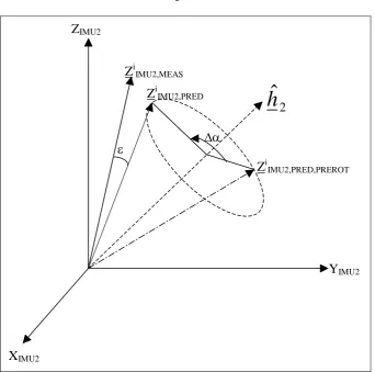
Figure 1 illustrates the predicted and measured Z inertial axis in the IMU2 frame. ZiIMU2,PRED,PREROT is the inertial vector before the rotation about the hinge axis hˆ2,
ZiIMU2,PRED is the same vector after the rotation as predicted by equation (11),
substituting Vi with [0 0 1]T, and ZiIMU2,MEAS is the measured vector as given by
equation (12). ε is the error angle between the predicted and measured vectors and it is present due to measurement errors in the IMU output Euler angles:
( )
iMEAS IMU i
PRED
IMU Z
Z 2, 2,
cosε = ⋅ (13)
Therefore, at each time step the knee angle is calculated to minimise the error angle ε in equation (13).
3. Experimental Validation
The test subjects were asked to stand still on the treadmill within the cameras’ capture volume and data were recorded for ten seconds (the static calibration trial). The
anatomical reflective markers were then removed leaving the markers on the IMUs as tracking markers for both the leg segments and the IMUs during the dynamic trials.
The IMUs, the camera system and a synchronisation unit were first connected via a cable. Following synchronisation of the systems, the cable was removed prior to the start of walking trials. . Subjects began walking on the treadmill at 1mile/hour and the speed was increased in five increments to 5miles/hour over a 5 minute period until the subject was running. The IMU and camera data were captured at 100Hz.
The roll, pitch and yaw angles that describe the rotation of the IMU reference frames with respect to an inertial frame were extracted from the Qualysis camera data using Visual 3D. The angles were represented in the Euler 3-2-1 sequence that the knee angle estimator requires for processing. From this camera derived data at the first time step, the initial rotation matrix between the IMU frames (
( )
02 1→
M ) was calculated.
This defines the absolute flexion/extension angle of the knee, i.e. the observed angle during the standing posture is taken to be a knee angle of 0. The knee rotation axis was defined from the camera derived data to be coincident with the anatomical flexion-extension axis of the knee (derived using anatomical landmarks) and was required to initialise the IMU based knee angle estimator.
reference frames with respect to a pseudo-inertial frame were estimated. Due to the inability of accelerometers and rate gyros alone to provide absolute orientation about the gravity vector (nominally the z inertial axis), no azimuth angle estimation was
provided. To avoid singularities in the estimation of the remaining Euler angles (pitch and roll about intermediate x and y axes), the algorithm automatically adjusted the
rotation sequence in each time step to either Euler 3-2-1 or Euler 3-1-2 (Appendix A). The outputs of the estimation namely the roll and pitch angles and the rotation sequences for the two IMUs at each time step were saved in a text file to be read by the knee joint angle estimator. The knee rotation axis and the initial rotation matrix between the two IMU frames were already known from the camera derived calibration information.
4. Results
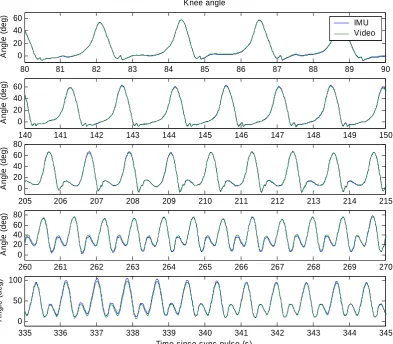
In this section the overall estimation performance is described by comparison with reference results calculated from the camera data. In figure 3, the knee angles estimated from camera and IMU data are compared for different speeds (only a subset of the data is shown). The vibration of the IMUs that occurs at heel strike is evident at knee angles close to zero.
bounded errors on inclination irrespective of the experiment duration, so the decrease in accuracy is likely to be due primarily to the waking/running speed.
Figure 5 shows the pitch and roll angles as measured by the IMU and the camera system for both the thigh and shank.
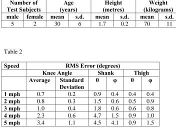
The RMS errors of the knee angle estimator for the entire data set are given in Table 2, along with the estimation errors produced by the EKF for both the shank and the thigh. It was observed that the knee angle estimation error is sometimes smaller than the errors in the individual angle measurements. Due to the physical mounting of the sensors the estimate of knee angle is mainly dependent on the estimates of φ, so errors in θ do not necessarily lead to errors in knee angle. Secondly, if there is any degree of correlation in the errors in thigh and shank measurements of φ, then the errors will partially cancel, leading to small knee angle errors.
5. Discussion
This study has demonstrated that two IMUs (attached to the thigh and shank), each consisting of a 3-axis accelerometer and three single axis rate gyroscopes, provide sufficient data to obtain high accuracy knee angle estimates. Kalman filters are used to estimate the pitch and roll of each IMU and this information, together with known anatomical constraints on knee joint motion, is used to estimate knee angle.
In the validation trials, knee angle was estimated over a 5 minute period with RMS errors of 0.7 deg for walking and 3.4 deg for running based on a single static
measure body segment orientation or joint angles, their validation experiments have used relatively slow movements or movements of short duration [11-13]. Furthermore, some researchers have compared their IMU results with less accurate validation
instrumentation than the methods used here (e.g. [14] [15]).
Luinge & Veltink [4] also produced promising results by using an IMU and Kalman filter to estimate orientation of the trunk, pelvis and forearm. Accuracy is increased by comparing (drift prone) gyro measurements with autocalibrated accelerometer
measurements [16] using knowledge of the frequency of movement and gravity. They achieved RMS errors of around 3 degrees; however, in the tasks they used for
validation (lifting & daily routine tasks), the body segments were relatively slow moving. Further research by Luinge et al [9] evaluated elbow joint orientation using a similar approach to the one described in this paper. Their method measured full joint orientation and included a practical calibration procedure, whereas our method simplified the knee joint to a single angle. However, their validation experiment was over a short duration (10-30 seconds) and had less dynamic movement in comparison to the running validation used here. In the results presented here (Table 2), RMS errors were less than 3 degrees for all cases except the fastest running speed.
flexion/extension. We assume that their errors would increase with the distance walked because of the integration of rate gyro biases.
An important limitation of the work presented in this paper is that the knee is assumed to be a perfect hinge joint, and hence while the flexion-extension angle is measured well, rotations about other axes are not estimated. This could be addressed by adding filters to estimate the remaining two angles, based on a model of the knee which allowed small deviations from 0 in these angles, but stipulated that the average angle was 0. A Kalman filter would probably work well here: the existing system would allow direct calculation of the rate-of-change of the remaining two knee angles (which would provide the measurements to the Kalman filter), and a simple stochastic
prediction model could be used to stabilise the system. This would allow a complete 3D estimate of the knee angle, albeit at the expense of some additional complexity.
A key question in the design of any EKF is stability. Both the experimental results and also long duration simulation based testing indicate that the filter is stable. However, this is dependent on the movement dynamics (acceleration, velocity and rate of rotation) remaining within the bounds specified in the filter parameters – higher dynamics lead to instability. One area that was not well tested by the
As is the case with alternative IMU based approaches (Favre [8] and Luinge & Veltink [4]), the performance of our system is dependent on the accuracy with which the initial calibration is performed. Further development work is required to eliminate the need for a camera system for calibration. An alternative static alignment
calibration method could be to take measurements from the IMUs with the test
subject’s body segments in known static orientations or joint angles. Greater accuracy could be obtained by combining these static measurements with some known dynamic movements, as proposed by Favre et al [8] and Luinge et al [9].
Acknowledgements
The authors would like to thank the European Commission for funding this research through the healthy aims program (IST FP6). In addition they would like to thank Mr Anmin Liu for his technical assistance with the Qualysis motion capture cameras.
Conflict of Interest Statement
No financial or personal relationships exist to create any conflict of interest for any of the authors who are affiliated to the University of Salford or to Analyticon. Diana Hodgins is the managing director and the owner of European Technology for
References
1. Kavanagh, J.J. and H.B. Menz, Accelerometry: a technique for quantifying movement patterns during walking. Gait Posture, 2008. 28(1): p. 1-15.
2. Orizio, C., Muscle sound: Bases for the introduction of a mechanomyographic
signal in muscle studies. Critical Reviews in Biomedical Engineering, 1993.
21(3): p. 201-243.
3. Plasqui, G. and K.R. Westerterp, Physical activity assessment with
accelerometers: an evaluation against doubly labeled water. Obesity (Silver
Spring), 2007. 15(10): p. 2371-9.
4. Luinge, H.J. and P.H. Veltink, Measuring orientation of human body segments
using miniature gyroscopes and accelerometers. Med Biol Eng Comput, 2005.
43(2): p. 273-82.
5. Roetenberg, D., et al., Compensation of magnetic disturbances improves
inertial and magnetic sensing of human body segment orientation. IEEE Trans
Neural Syst Rehabil Eng, 2005. 13(3): p. 395-405.
6. de Vries WH, Veeger HE, Baten CT, van der Helm FC, Magnetic distortion in motion labs, implications for validating inertial magnetic sensors. Gait
Posture. 2009 Jun;29(4):535-4
7. Favre, J., et al., Quaternion-based fusion of gyroscopes and accelerometers to improve 3D angle measurement. Electronics Letters, 2006. 42(11): p. 612-614.
8. Favre, J., et al., Ambulatory measurement of 3D knee joint angle. J Biomech,
2008. 41(5): p. 1029-35.
10. Cui, C.K. and G. Chen, Kalman filtering: with real time applications. 3rd ed.
1999: Springer.
11. Boonstra MC et al., The accuracy of measuring the kinematics of rising from a
chair with accelerometers and gyroscopes. Journal of Biomechanics, 2006. 39
p. 354-358
12. Tong K and Granat MH, A practical gait analysis system using gyroscopes.
Medical Engineering & Physics, 1999. 21 p. 87-94
13. Huddleston J et al. Ambulatory measurement of knee motion and physical
activity: preliminary evaluation of a smart activity monitor. Journal of
NeuroEngineering and Rehabilitation, 2006. 3(21)
14. Dejnabadi H et al. Estimation and visualisation of sagittal kinematics of lower
limbs orientation using body-fixed sensors. IEEE Transactions on Biomedical
Engineering, 2006. 53(7) p. 1385-1393
15. Williamson R and Andrews BJ. Detecting absolute human knee angle and
angular velocity using accelerometers and rate gyroscopes. Medical Biology
and Engineering Computing, 2001. 39(3) p. 294-302
16. Luinge, H.J. and P.H. Veltink, Inclination measurement of human movement
using a 3D accelerometer with autocalibration. IEEE Trans. Neural Syst.
Figure 1
2
ˆ
h
Δα
ZiIMU2,PRED,PREROT ZiIMU2,PRED
ZiIMU2,MEAS
ε ZIMU2
XIMU2
Figure 3
80 81 82 83 84 85 86 87 88 89 90
0 20 40 60 S e tti n g 1 A n gle ( d eg ) Knee angle IMU Video
140 141 142 143 144 145 146 147 148 149 150 0 20 40 60 Se tt in g 2 A ng le ( d eg )
205 206 207 208 209 210 211 212 213 214 215 0 20 40 60 80 S e tti n g 3 A ng le ( d eg )
260 261 262 263 264 265 266 267 268 269 270 0 20 40 60 80 S e tti n g 4 A n gl e ( d eg)
335 336 337 338 339 340 341 342 343 344 345 0 50 100 S e tti n g 5 A ngl e (d eg )
Figure 4
80 81 82 83 84 85 86 87 88 89 90
-2 0 2 S et ti ng 1 E rro r (d e g ) Knee angle
140 141 142 143 144 145 146 147 148 149 150 -4 -2 0 2 4 S e tti n g 2 E rro r ( d e g )
205 206 207 208 209 210 211 212 213 214 215 -5 0 5 S e tti n g 3 E rr o r (d e g )
260 261 262 263 264 265 266 267 268 269 270 -5 0 5 S e tti n g 4 E rro r (d e g )
335 336 337 338 339 340 341 342 343 344 345 -10 0 10 S e tti n g 5 E rro r (d e g )
Figure 5
(b) Shin IMU (a) Thigh IMU
An
g
le
(de
g)
g
le
(de
g)
An
g
le
(de
g)
An
g
le
(de
g)
An
time (s) time (s)
(d) Shin Video (c) Thigh Video
Figure 1: Graphical representation of the Z inertial vectors in the IMU2 frame
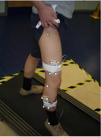
Figure 2: IMU and reflective marker position on the test subject. Two IMUs (one on the thigh, one on the shank) were attached to each test subject. The IMUs each had 4 markers to enable the camera system to record their position and orientation. The knee axis was defined by markers on the two epicondyles and markers were also placed on the malleoli and the greater trochanter.
Figure 3: Comparison of knee angle estimates using camera and IMU data for Subject 1 at speeds of 1mph (top graph) to 5mph (bottom graph).
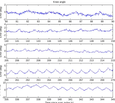
Figure 4: Knee angle estimation error from camera and IMU data for Subject 1 at speeds of 1mph (top graph) to 5mph (bottom graph).
Figure 5: Euler angles measured by the IMU and the camera system for both the thigh and shank (shin) body segments.
Table 1: Test subject anthropometric data (note that s.d. refers to standard deviation)
Table 1 Number of Test Subjects
Age (years)
Height (metres)
Weight (kilograms) male female mean s.d. mean s.d. mean s.d.
[image:27.595.82.435.102.364.2]5 2 30 6 1.7 0.2 70 11
Table 2
Speed RMS Error (degrees)
Knee Angle Shank Thigh Average Standard
Deviation
θ φ θ φ
APPENDICES
A. Avoiding singularities by switching between Euler formulations
The Euler 321 formulation has singularities at . An alternative Euler
formation which still allows the angle
o
90
± =
θ
ψˆ to be kept separate from the rest of the state
vector is the 312 formulation, with singularities at . The software can avoid
these singularities by switching between formulations when the angles in the current formulation get too close to the singularities.
o 90
± =
φ
B. Choice of Euler angle representation
The yaw angle ψ cannot be known accurately, because it is the angle of rotation
around the z-axis, i.e. rotation around the gravity vector (estimate of the change in
azimuth since switch on). Therefore, the angle ψ is separate from the state vector, and
is assumed by the filter to have zero error in its estimation. Let ψˆ be the filter’s “zero
error” estimation of ψ. The propagation equations for θ and φ are independent of ψˆ .
Therefore, the pseudo inertial frame is defined as the inertial frame rotated around the gravity vector by an arbitrary (and generally unknown) amount. Specifically, the yaw
angle relating the sensor and the pseudo inertial frames is ψˆ , whereas the yaw angle
relating the sensor and true inertial frames is ψ. Using Euler angles allows ψ to be
C. Derivation of MROT
The matrix MROT
( )
t describes the transformation of a vector in the IMU2 frame attime zero to the IMU2 frame at time t after a rotation about the knee hinge axis unit
vector hˆ2 in the IMU2 frame. Assuming that the difference in knee angle at time zero
and at time t is Δα(t), the rotation about the hinge vector can be described by a unit
quaternion, equation (A1)
( )
( )
( )
( )
( )
( )
( )
( )
( )
⎥⎥ ⎥ ⎥ ⎦ ⎤ ⎢ ⎢ ⎢ ⎢ ⎣ ⎡ = ⎥ ⎥ ⎥ ⎥ ⎥ ⎥ ⎥ ⎥ ⎥ ⎦ ⎤ ⎢ ⎢ ⎢ ⎢ ⎢ ⎢ ⎢ ⎢ ⎢ ⎣ ⎡ ⎟ ⎠ ⎞ ⎜ ⎝ ⎛ Δ ⎟ ⎠ ⎞ ⎜ ⎝ ⎛ Δ ⎟ ⎠ ⎞ ⎜ ⎝ ⎛ Δ ⎟ ⎠ ⎞ ⎜ ⎝ ⎛ Δ = t q t q t q t q t h t h t h t t q Z Y X rot 0 3 2 1 , 2 , 2 , 2 2 cos ˆ 2 sin ˆ 2 sin ˆ 2 sin α α α α (A1)The unit hinge vector retains the same orientation in the IMU2 frame throughout time since, as explained earlier no residual movements due to muscle activity and loose skin are taken into account. The corresponding rotation matrix that describes the mapping of a vector between the IMU2 frames before and after the above rotation is given from quaternion algebra, equation (A2)
( )
⎥ ⎥ ⎥ ⎦ ⎤ ⎢ ⎢ ⎢ ⎣ ⎡ + − − − + + − + − − − + − − + = 2 3 2 2 2 1 2 0 1 0 3 2 2 0 3 1 1 0 3 2 2 3 2 2 2 1 2 0 3 0 2 1 2 0 3 1 3 0 2 1 2 3 2 2 2 1 2 0 2 2 2 2 2 2 2 2 2 2 2 2 q q q q q q q q q q q q q q q q q q q q q q q q q q q q q q q q q q q q tMROT (A2)
Note that the use of a quaternion formulation in this part of the derivation is simply because it is a convenient way to describe and calculate a rotation of a specified angle,
( )
tα