An efficient energy storage & return prosthesis

Full text

(1)AN EFFICIENT ENERGY STORAGE & RETURN PROSTHESIS. Abu Zeeshan Bari. Ph.D. Thesis. 2013.

(2) AN EFFICIENT ENERGY STORAGE & RETURN PROSTHESIS. Abu Zeeshan Bari. Centre for Health Sciences Research University of Salford, Salford, UK. Submitted in Partial Fulfilment of the Requirements of the Degree of Doctor of Philosophy, March 2013.

(3) Dedicated to my late parents, who taught me how to read and write..

(4) TABLE OF CONTENTS TABLE OF CONTENTS. IV. LIST OF FIGURES. IX. LIST OF TABLES. XV. NOMENCLATURE. XVII. ACKNOWLEDGEMENTS. XXI. DECLARATION. XXII. ABSTRACT. XXIII. 1. INTRODUCTION. 1. 2. LITERATURE REVIEW. 4. 2.1 Healthy Gait ...............................................................................................4 2.1.1 Metabolic Cost of Walking ..................................................................5 2.1.2 Mechanical Analysis of Human Energetics .........................................8 2.1.3 Gait Efficiency .....................................................................................9 2.2 Gait Models ................................................................................................9 2.3 Role of Ankle in Anatomically Intact Gait ............................................13 2.3.1 Ankle Kinetics....................................................................................15 2.4 Amputee Gait ...........................................................................................17 2.4.1 Energy Efficiency of Amputee Gait...................................................17 2.5 Current Prosthetic Feet...........................................................................19 2.5.1 Conventional & Energy Storing/Return Prosthetic Feet ....................19 2.5.2 Review of Studies on Comparing Different Prosthetic Feet and Their Effect on Amputee Gait ............................................................20 2.5.3 Gait Deviations at the Ankle in Amputees.........................................23 2.5.4 Proposed Reasons for Low Energy Efficiencies ................................25. iv.

(5) 2.6 Previous Attempts to Address the Problems of Energy Efficiency in Transtibial Amputee Gait ...................................................................26 2.6.1 Active Prostheses ...............................................................................26 2.6.1.1. Pneumatically Actuated Devices .......................................26. 2.6.1.2. Electrically Actuated Devices ............................................29. 2.6.1.3. Quasi-Passive Devices .......................................................31. 2.6.1.4. Summary of Active Prostheses ..........................................33. 2.7 Alternative Actuation Technologies .......................................................34 Flywheels ............................................................................................36 Hydraulic Accumulators .....................................................................36 Batteries ..............................................................................................37 Super capacitors ..................................................................................37 2.8 Conclusions...............................................................................................39 3. CONCEPT DESIGN I. 41. 3.1 Overview ...................................................................................................42 3.2 System Components ................................................................................45 3.2.1 Variable Displacement Actuator ........................................................45 3.2.2 Hydraulic Accumulator ......................................................................47 3.2.3 Spring-Loaded Accumulator ..............................................................48 3.2.4 Gas-Charged Accumulators ...............................................................48 3.2.5 Pressure Relief Valve .........................................................................49 3.3 Modelling and Sizing of Hydraulic Accumulator .................................50 3.3.1 Definitions of Accumulator Parameters .............................................50 a) Pre-charge Pressure .......................................................................51 b) Maximum Rated Pressure .............................................................52 c) Minimum Rated Pressure ..............................................................52 d) Compression Ratio ........................................................................52 e) Accumulator Capacity ...................................................................53 f) Instantaneous Oil Volume .............................................................53 3.3.2 Energy Stored Over a Gait Cycle .......................................................53 v.

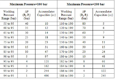
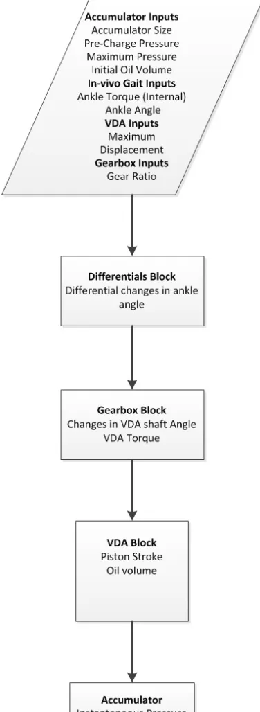
(6) 3.3.3 Developing Equations for Sizing a Spring-Loaded Accumulator .....55 a) General Case..................................................................................55 b) Spring-loaded Accumulator ..........................................................56 3.3.4 Spring-Loaded Accumulator-Sizing and Selection ............................61 a) Case 1: ...........................................................................................62 b) Case 2: ...........................................................................................63 3.3.5 Developing Equations for Sizing a Gas-Charged Accumulator ........64 3.3.6 Gas-Charged Accumulator-Selection and Sizing ..............................70 a) Case 1: ...........................................................................................70 b) Case 2: ...........................................................................................71 3.4 Modelling of Variable Displacement Pump/Motor ..............................73 3.4.1 Ideal VDA Model...............................................................................74 3.4.2 VDA Loss Model ...............................................................................74 3.5 Modelling of Gearbox ..............................................................................77 3.6 System Simulation ...................................................................................80 3.6.1 Differentials and Gearbox Blocks ......................................................83 3.6.2 VDA Block ........................................................................................85 3.6.3 Accumulator Block ............................................................................86 a) Spring-Loaded accumulator ..........................................................86 b) Gas-Charged accumulator .............................................................87 3.7 Design Simulations ..................................................................................88 3.7.1 VDA Sizing – Ideal Conditions .........................................................90 3.7.2 VDA/Gearbox Sizing - Real Conditions ............................................92 3.8 Pseudo Control .........................................................................................96 3.9 System Testing .......................................................................................103 3.9.1 Level Walking ..................................................................................105 a) Salford’s Gait Data ......................................................................105 a) Data from Lay et al, 2006............................................................105 3.9.2 Decline Walking ..............................................................................107 b) 8.5° Decline .................................................................................108 vi.

(7) c) 21° Decline ..................................................................................111 3.9.3 Incline Walking ................................................................................113 a) 8.5° Incline ..................................................................................114 b) 21° Incline ...................................................................................117 3.9.4 Summary ..........................................................................................119 3.10 Discussion ...............................................................................................120 3.10.1 System Performance ........................................................................121 3.10.2 Feasibility .........................................................................................123 4. CONCEPT DESIGN II. 126. 4.1 Overview of example design .................................................................128 4.1.1 Actuation Concept I .........................................................................129 4.1.2 Actuation Concept II ........................................................................134 4.2 Mechanics ...............................................................................................136 4.3 System Simulation .................................................................................143 4.3.1 Independent Inputs Block ................................................................146 4.3.2 Coefficients Block............................................................................146 4.3.3 Quartic Block ...................................................................................147 4.3.4 Mechanics Block ..............................................................................148 4.3.5 Differentials Block ...........................................................................149 4.3.6 Gearbox Block .................................................................................150 4.3.7 VDA and Cylinder Block .................................................................151 4.3.8 Accumulator Block ..........................................................................154 4.4 Design Simulations ................................................................................154 4.4.1 Method of Finding Optimum values of Design Variables-Ideal Conditions ........................................................................................155 4.4.2 VDA/Gearbox Sizing- Real Conditions ...........................................157 4.5 System Testing .......................................................................................159 4.5.1 Level Walking ..................................................................................160 b) Salford’s Gait Data ......................................................................160 c) Data from Lay et al, 2006............................................................163 vii.

(8) 4.5.2 Decline Walking ..............................................................................165 a) 8.5° Decline .................................................................................166 b) 21° Decline ..................................................................................169 4.5.3 Incline Walking ................................................................................172 a) 8.5° Incline ..................................................................................172 b) 21° Incline ...................................................................................175 4.5.4 Summary ..........................................................................................177 4.6 Discussion ...............................................................................................178 4.6.1 System Performance ........................................................................178 4.6.2 Feasibility .........................................................................................180 5. CONCLUSION. 183. 5.1 Summary ................................................................................................183 5.2 Novel Contributions ..............................................................................187 5.3 Limitations .............................................................................................187 5.4 Main Conclusions ..................................................................................188 5.5 Future Work ..........................................................................................189 APPENDIX-A. 190. APPENDIX-B. 191. APPENDIX-C. 193. APPENDIX-D. 196. REFERENCES. 197. viii.

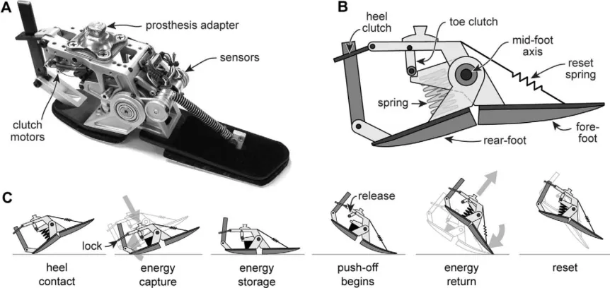
(9) LIST OF FIGURES Figure 2.1: A normal gait cycle. ..............................................................................4 Figure 2.2: Energy cost of walking as a function of speed. .....................................6 Figure 2.3: Minimum energy cost of walking as a function of slope. .....................7 Figure 2.4: Illustration of COM trajectories by the inverted pendulum model. ....10 Figure 2.5: Inverted pendulum model....................................................................12 Figure 2.6: Ankle angle, internal moment, and power data for healthy individuals. ..........................................................................................14 Figure 2.7: Ultrasound imaging data from human walking showing the instantaneous power for gastrocnemius muscle fibres and Achilles tendon. .................................................................................................16 Figure 2.8: Reported energy cost for transtibial amputees (scattered plot) at self-selected walking speeds. ..............................................................18 Figure 2.9: Reported energy cost for transfemoral amputees (scattered plot) at self-selected walking speeds. ..............................................................19 Figure 2.10: Energy cost for transtibial amputees (scattered plot) using different commercially available prosthetic feet at self-selected walking speeds. ...................................................................................22 Figure 2.11: Comparison of gait parameters between a healthy individual and a transtibial amputee. ..........................................................................23 Figure 2.12: Schematic diagram of the pneumatic actuator. .................................27 Figure 2.13: A) Prototype device. (B) Schematic design. (C) Working sequence. .............................................................................................32. ix.

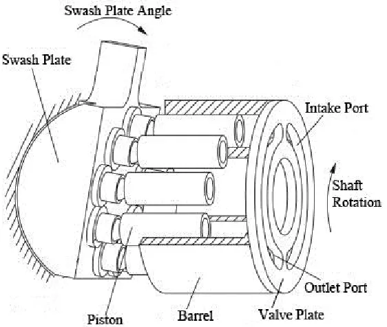
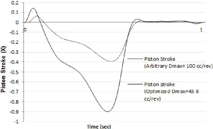
(10) Figure 2.14: Hatched area corresponding to the stored and released energy by the energy recycling foot.....................................................................32 Figure 3.1: Schematic diagram of the concept design. ..........................................44 Figure 3.2: Schematic diagram of a variable displacement pump/motor. .............46 Figure 3.3: Gas-charged accumulator (left) and Spring-loaded accumulator (right). .................................................................................................48 Figure 3.4: Energy stored over a gait cycle. ..........................................................54 Figure 3.5: An arbitrary pressure profile of an accumulator. ................................55 Figure 3.6: Pressure profile of a spring-loaded accumulator. ................................56 Figure 3.7: Pressure-volume relationship for a gas-charged accumulator. ............66 Figure 3.8: Simulink circuit for concept design I. .................................................81 Figure 3.9: Simulation process flow. .....................................................................82 Figure 3.10: Piston Stroke (X) obtained from first simulation run with an arbitrary Dmax and from an optimized Dmax obtained as results of an iterative process. .............................................................................91 Figure 3.11: Final accumulator pressure for Dmax and N. ......................................94 Figure 3.12: An ankle power profile sample compared with the effect of the control system. ....................................................................................97 Figure 3.13: Energy profiles for the original ankle power data and for the reduced power data. ............................................................................98 Figure 3.14: Accumulator pressures obtained with a gas-charged accumulator for ideal and real conditions. ...............................................................99 Figure 3.15: Accumulator pressures obtained with a gas-charged accumulator for ideal, real, and real scaled conditions using Salford’s gait data. .100 x.

(11) Figure 3.16: Torque profile for ideal and real scaled conditions using Salford’s gait data. ............................................................................102 Figure 3.17: Power profile for ideal and real scaled conditions using Salford’s gait data. ............................................................................................102 Figure 3.18: Pressure profile for ideal, real, and real scaled conditions using level walking data from Lay et al., 2006...........................................105 Figure 3.19: Torque profile for ideal and real scaled conditions using level walking data from Lay et al., 2006. ..................................................106 Figure 3.20: Power profile for ideal and real scaled conditions using level walking data from Lay et al., 2006. ..................................................107 Figure 3.21: Pressure profile for ideal, real, and real scaled conditions using 8.5° decline walking data from Lay et al., 2006. ..............................108 Figure 3.22: Torque profile for ideal and real scaled conditions using 8.5° decline walking data from Lay et al., 2006. ......................................109 Figure 3.23: Power profile for ideal and real scaled conditions using 8.5° decline walking data from Lay et al., 2006. ......................................110 Figure 3.24: Pressure profile for ideal and real conditions using 21° decline walking data from Lay et al., 2006. ..................................................111 Figure 3.25: Torque profile for ideal and real conditions using 21° decline walking data from Lay et al., 2006. ..................................................112 Figure 3.26: Power profile for ideal and real conditions using 21° decline walking data from Lay et al., 2006. ..................................................113 Figure 3.27: Pressure profile for ideal, real, and real scaled conditions using 8.5° incline walking data from Lay et al.,2006. ................................114 xi.

(12) Figure 3.28: Torque profile for ideal and real scaled conditions using 8.5° incline walking data from Lay et al., 2006. ......................................115 Figure 3.29: Power profile for ideal and real scaled conditions using 8.5° incline walking data from Lay et al., 2006. ......................................116 Figure 3.30: Pressure profile for ideal, real, and real scaled conditions using 21° incline walking data from Lay et al., 2006. ................................117 Figure 3.31: Torque profile for ideal and real scaled conditions using 21° incline walking data from Lay et al., 2006. ......................................118 Figure 3.32: Power profile for ideal and real scaled conditions using 21° incline walking data from Lay et al., 2006. ......................................119 Figure 4.1: A simple block diagram of an alternative design approach. .............127 Figure 4.2: Conceptual sketch of design II showing only the slider-crank spring mechanism. ............................................................................128 Figure 4.3: A simple hydraulic circuit with actuation concept I..........................130 Figure 4.4: Pressures for positive work phases. ...................................................131 Figure 4.5: Pressures for negative work phases. ..................................................132 Figure 4.6: Alternate circuit to control actuator torque during negative work phases. ...............................................................................................133 Figure 4.7: A simple hydraulic circuit for concept design II with VDA and gearbox. .............................................................................................135 Figure 4.8: Free body diagrams showing forces acting on the cylinder and footplate. ...........................................................................................137 Figure 4.9: Geometry diagram with forces acting on the cylinder. .....................139 Figure 4.10: Simulink circuit for concept design II. ............................................144 xii.

(13) Figure 4.11: A simplified flow chart for the calculation process for concept design II.............................................................................................145 Figure 4.12: Optimum values of design variables for concept design II. ............156 Figure 4.13: Final accumulator pressure for Dmax and N. ....................................157 Figure 4.14: Pressure profile obtained for ideal, real, and real scaled conditions for Salford’s gait data. .....................................................160 Figure 4.15: Torque profile obtained for ideal and real scaled conditions for Salford’s gait data. ............................................................................161 Figure 4.16: Power profile obtained for ideal and real scaled conditions for Salford’s gait data. ............................................................................162 Figure 4.17: Pressure profile obtained for ideal, real, and real scaled conditions for level walking data from Lay et al., 2006. ..................163 Figure 4.18: Torque profile obtained for ideal and real scaled conditions for level walking data from Lay et al., 2006...........................................164 Figure 4.19: Power profile obtained for ideal and real scaled conditions for level walking data from Lay et al., 2006...........................................165 Figure 4.20: Pressure profile obtained for ideal and real conditions for 8.5° decline data from Lay et al., 2006. ....................................................166 Figure 4.21: Torque profile obtained for ideal and real conditions for 8.5° decline data from Lay et al., 2006. ....................................................167 Figure 4.22: Power profile obtained for ideal and real conditions for 8.5° decline data from Lay et al., 2006. ....................................................168 Figure 4.23: Pressure profile obtained for ideal and real conditions for 21° decline data from Lay et al., 2006. ....................................................169 xiii.

(14) Figure 4.24: Torque profile obtained for ideal and real conditions for 21° decline data from Lay et al., 2006. ....................................................170 Figure 4.25: Power profile obtained for ideal and real conditions for 21° decline data from Lay et al., 2006. ....................................................171 Figure 4.26: Pressure profile obtained for ideal and real conditions for 8.5° incline data from Lay et al., 2006. ....................................................172 Figure 4.27: Torque profile obtained for ideal and real conditions for 8.5° incline data from Lay et al., 2006. ....................................................173 Figure 4.28: Power profile obtained for ideal and real conditions for 8.5° incline data from Lay et al., 2006. ....................................................174 Figure 4.29: Pressure profile obtained for ideal and real conditions for 21° incline data from Lay et al., 2006. ....................................................175 Figure 4.30: Torque profile obtained for ideal and real conditions for 21° incline data from Lay et al., 2006. ....................................................176 Figure 4.31: Power profile obtained for ideal and real conditions for 21° incline data from Lay et al., 2006. ....................................................177. xiv.

(15) LIST OF TABLES Table 2.1: Comparison of energy storage technologies. ........................................38 Table 3.1: Spring-loaded accumulator capacities obtained for different working pressure ranges for maximum rated pressures of 100 and 200 bar.................................................................................................63 Table 3.2: Sizing results (rounded values) for gas-charged accumulators. ...........72 Table 3.3: Gearbox efficiency data obtained for a commercial gearbox ...............78 Table 3.4: Optimized size of the VDA obtained from simulation for both the spring-loaded and gas-charged accumulator type for ideal conditions. ...........................................................................................92 Table 3.5: VDA and gearbox sizes obtained for different accumulator sizes and types. ............................................................................................95 Table 3.6: Summary of optimum VDA and gearbox sizes for the test data. .......104 Table 3.7: Summary of peak power delivered by the system against the required peak power for the gait data used. ......................................120 Table 3.8: A weight comparison of VDA and VDA/gearbox sizes obtained for ideal and real models for the test data with similar commercially available components. ................................................124 Table 4.1: Design Variables used for ideal and real model. ................................158 Table 4.2: Comparison of VDA/VDA-gearbox sizes obtained for design II and compared with those obtained for design I. ...............................158 Table 4.3: Comparison of performance of design I and design II. ......................178. xv.

(16) Table 4.4: A weight comparison of VDA and VDA/gearbox sizes obtained for ideal and real models for the test data with similar commercially available components for design II. ...........................181. xvi.

(17) NOMENCLATURE ∆E. Total energy stored over one gait cycle. B. Bulk modulus of oil. C1. Coefficient of the 4th order term of the quartic equation. C2. Coefficient of the 3rd order term of the quartic equation. C3. Coefficient of the 2nd order term of the quartic equation. C4. Coefficient of the 1st order term of the quartic equation. C5. Coefficient of the zero order term of the quartic equation. Cs. Slip coefficient. Dact or D. Actuator’s instantaneous volumetric displacement. d. Slider position. dA. Differential changes in ankle angle. dAvda. Differential changes in gearbox output shaft rotation. dAgb. Differential changes in gearbox input shaft rotation. dβvda. Differential changes in VDA shaft angle. Dia. Cylinder bore. dl. Differential changes in cylinder stroke. Dmax. Actuator’s maximum volumetric displacement. dVvdaideal. Differential changes in oil volume of VDA for ideal conditions. dVvdareal. Differential changes in oil volume of VDA for real conditions. dVcyl. Differential changes in oil volume of cylinder. dVFideal. Differential changes in oil volume of accumulator for ideal case. dVFreal. Differential changes in oil volume of accumulator for real case. dβ. Differential changes in the shaft angle xvii.

(18) F1. Piston force due to accumulator pressure. F2:. Component of the force F (acting perpendicular to F1). k. Specific heat ratio. Km. Machine type coefficient. l. Cylinder length. Mact. Actuator Moment. Mank. Ankle moment. N. Gear ratio. n, a, b. Coefficients for the flow loss model. P or Pacc. Instantaneous accumulator pressure. Patm. Atmospheric Pressure. Ph. Higher working pressure. Pl. Lower working pressure. Pmax. Maximum rated pressure. Pmin. Minimum rated pressure. Ppr. Pre-charge pressure. q. Instantaneous flow rate. qvdaideal. Ideal actuator flow rate. qcompressibility. Flow loss due to compressibility. qideal. Ideal flow rate. qleakage. Leakage flow. qreal. Flow rate obtained with real conditions. qvdareal. Real actuator flow rate. T or Tvda. Instantaneous actuator torque. Tfr. Gearbox friction torque xviii.

(19) Tideal. Torque output for ideal conditions. TN. Nominal torque. Treal. Torque output for real conditions. VA. Accumulator capacity/size. VF. Instantaneous accumulator oil volume. VG. Gas volume. Vh. Higher working oil volume. Vhg. Higher working gas volume. Vl. Lower working oil volume. Vlg. Lower working gas volume. Vmax. Maximum oil volume. Vmin. Minimum oil volume. Voil. Useable oil volume. Vpr. Maximum gas volume (also equal to VA). Vr. Volume ratio. X. Actuator’s instantaneous stroke. Xmax. Actuator’s maximum stroke. x,y. Actuator Position. Xmax. Actuator’s maximum stroke. α. Ankle Angle. β. Actuator shaft angle. μ. Absolute viscosity of oil. ω. Ankle’s angular velocity. ωgb. Gearbox input shaft angular velocity. ωvda. VDA angular velocity xix.

(20) ωmax. Maximum VDA shaft angular velocity. xx.

(21) ACKNOWLEDGEMENTS I am deeply indebted to my trio of supervisors, Professor David Howard and Drs Laurence Kenney and Martin Twiste, who as a team, kept this thesis on track through to completion with their endless support, intellectual guidance, and enduring patience. Indeed, without their extraordinary guidance, this thesis would not be possible. I would like to thank Dr. Richard Jones for his help on certain aspects of this work. I offer my sincere gratitude to Rachel Shuttleworth for all her support and to my office colleagues for the stimulating discussions. I am highly grateful to my teachers at the NED University of Engineering & Technology, Pakistan, especially Prof. Dr. Muzaffar Mahmood and Prof. Neelofur Master, for being excellent educators, a constant source of inspiration, and for instilling in me a love of creative pursuits in science. I feel extremely privileged to have been their student. I extend my gratitude to the NED University of Engineering & Technology, for the grant of fellowship and study leave to pursue this work. I am deeply thankful to my siblings for their support and prayers when they were most needed. This last word of acknowledgment I have saved for my dear wife Saira, who has happily shared all my burdens without a complaint, and my son Ali, who has been a constant source of motivation for this work.. xxi.

(22) DECLARATION I declare that this thesis has been composed by myself and embodies the results of my own course of study and research whilst attending the University of Salford from January 2009 to March 2013. All sources and material have been acknowledged.. xxii.

(23) ABSTRACT Amputee gait is characterised by a higher metabolic cost of walking compared with anatomically intact subjects. Anatomically intact gait kinetics reveals that tendons crossing the ankle joint store and return strain energy during the stance phase of walking to provide forward propulsion. One of the main reasons for the high-energy cost of amputee gait is that passive prosthetic feet store little energy compared with the equivalent human structure and hence cannot provide the required energy at push-off. In addition, passive prosthetic feet are uncontrolled in the storage and release of strain energy, and do not provide natural levels of resistance and propulsion. Therefore, designing a passive prosthesis to efficiently store and transfer energy between joints, with continuous control over ankle torque, remains a research challenge. With the aim of developing an energy efficient passive prosthesis capable of mimicking the controlled energy recycling behaviour seen in an anatomically intact limb, a hydraulics-based design was investigated in this work. A first design concept, based on a hydraulic accumulator, a variable displacement hydraulic actuator (VDA), a gearbox, and a low-pressure oil tank, was developed. The accumulator served as energy storage medium, where VDA served as the only actuator to provide ankle torque. Simulation showed that the design outperformed commercial passive prostheses as well as a recent novel design based on a spring-clutch mechanism. For level walking, it provided 86% and 69% of the peak power required by the anatomical ankle whilst providing near normal ankle torques. The system was able to store all of the available energy during gait and provide correctly timed release of energy. However, a feasibility study showed problems with size and weight of a potential prototype.. xxiii.

(24) To address this problem a second design was developed with the aim of reducing the size and weight of VDA in design I. The second design comprised of a spring to provide ankle torque and to reduce the torque load on the VDA. The spring is connected to the ankle via a lever arrangement, and the VDA is used to vary the lever arm to continuously control ankle torque. Simulation results showed that design II outperformed design I; it delivered higher values of peak power, and a feasibility study showed that, using bespoke component designs, it might be possible to incorporate it into a lower limb prosthesis.. xxiv.

(25) 1. INTRODUCTION During the stance phase of gait, the ankle contributes 60% of the positive mechanical work performed collectively by the ankle, knee and hip joint and majority of this work is provided by a release of strain energy (stored earlier in gait) through tendons crossing the ankle joint (Sawicki et al., 2009). Therefore, utilizing the spring-like behaviour of the tendons by using a compliant prosthetic foot might restore near to the anatomically intact ankle work. In order to provide similar ankle mechanical work, a prosthetic foot must satisfy three requirements: a) resist both plantarflexion and dorsiflexion in load acceptance and mid-stance; b) assist plantarflexion and resist dorsiflexion in late stance; and c) assist dorsiflexion in swing without consuming unnecessary amount of energy (Winter, 2004a). A summary of these requirements is that the prosthetic foot should provide natural levels of resistance and propulsion. In other words, the compliant elements of the prosthesis must store and release energy (whilst providing near to the anatomically intact ankle torques) at the right instant during the gait cycle. Commercially available energy storage and return (ESR) prostheses do not meet these requirements pertaining to the uncontrolled energy storage/release by their compliant elements. For instance, an anatomically intact ankle resists the initial plantarflexion and subsequent dorsiflexion during load acceptance and mid-stance respectively, due to eccentric contraction of the relevant muscles and tendons, resulting in a build-up of strain energy in relevant tendons. In turn, in a passive ESR prosthesis, the strain energy stored in the rear foot during load acceptance is released during mid-stance (when an anatomically intact foot is storing energy while resisting dorsiflexion), thus failing to satisfy requirement (a) set out above. 1.

(26) In late stance, by the time when an anatomically intact limb releases its stored energy to assist plantarflexion, the ESR prosthesis, having dissipated all the stored energy earlier, does not assist the late stance plantarflexion (and so, do not assist in forward propulsion of the limb). Furthermore, at push-off, as the load increases, the prosthetic foot dorsiflexes at a point in time when an anatomically intact foot would be plantarflexing. Designing a passive prosthesis that could utilize the passive energy storage and return behaviour observed in an anatomically intact ankle remains a research challenge. Therefore, the aim of the work described here was to develop a design concept that is able to mimic the energy recycling behaviour as seen in anatomically intact gait. Hydraulics based design concepts were investigated as hydraulics allowed for continuous control, and high-density energy storage/transfer between joints. This thesis addresses three objectives: 1- Identify efficient means of energy storage and return mechanism as observed in an anatomically intact gait. 2- Based on the understanding of energy flows at a joint level, develop a passive prosthesis (with controlled energy storage and return mechanisms) through modelling, while considering feasibility for developing a prototype. 3- Virtual testing of the prosthesis using published gait data for level, declined, and inclined walking. The novel contributions of this work were the development of two concept designs utilizing hydraulics technology that were shown to be capable of efficiently storing and returning energy with continuous control of ankle torque. In addition, this was the first study to show that a conceptual prosthetic design based on hydraulics is practically feasible and 2.

(27) could equal the performance of an actively powered prosthesis over level ground and decline walking.. The remainder of this thesis is separated into four chapters. Chapter 2 provides a basis for studying gait efficiency in anatomically intact and amputee gait, including the role of the ankle for an efficient gait, prosthesis design, and previous approaches to improve the energy efficiency in transtibial amputee gait. Chapter 3 describes the development. of. a. new. model. for. an. energy. efficient. prosthesis,. with. definition/description of the components used, including the development of mathematical equations for the components used in the model, their sizing, and selection, and then testing of the model using gait data. Based on the results obtained from the first design, Chapter 4 presents another approach to further improve the first design in terms of size and weight, working principle, modelling, and simulation and testing of the model. This is followed by Chapter 5, which provides an overall discussion on the aims and objectives, findings of the work, novel contributions, limitations, and future work.. 3.

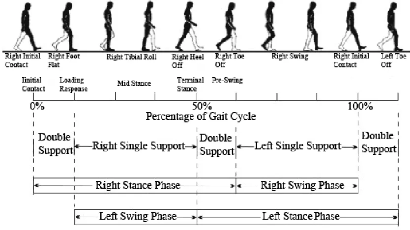
(28) 2. LITERATURE REVIEW 2.1 Healthy Gait Human gait is a complex biomechanical phenomenon involving forward progression of the body in a controlled manner. The term “gait cycle” refers to the time elapsed between two identical gait events, typically the instant of one of the feet making ground contact (Whittle, 2003). With this definition, the gait cycle is divided into two major phases; stance and swing. Stance phase, during which the foot remains in contact with the ground, typically makes up 60% of the gait cycle. Swing phase involves the forward progression of the limb, during which the foot leaves the ground, and typically makes up the remaining 40% of the gait cycle. When both feet are in contact with the ground, the period is called double support (Rose & Gamble, 2006). An overview of the gait cycle is shown in Figure 2.1.. Figure 2.1: A normal gait cycle. Figure adapted from Racic et al., 2009. 4.

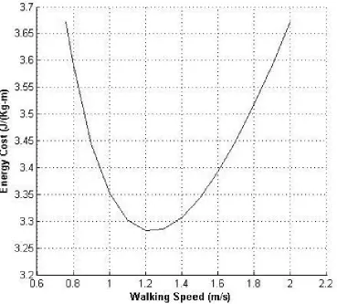
(29) 2.1.1. METABOLIC COST OF WALKING Taking into account that aerobic metabolism requires burning up of. carbohydrates, fats and proteins in the presence of oxygen, metabolic energy expenditure can be indirectly calculated by measuring the volume of oxygen intake (VO2) (Kirtley, 2006). As metabolic energy expenditure increases with body mass to allow for comparison between subjects, energy expenditure values are typically presented as normalized by body mass. Energy expenditure can be represented either as a time rate of oxygen (termed as “O2 Rate” with typical units of ml/(kg.min)), or as oxygen consumed per unit distance (termed as “O2 Cost” with typical units of ml/(kg.m)). Using an energy equivalent of 21.1 J for one ml of O2 as defined by Brockway, 1987, the O2 cost can be represented as energy cost with units of J/(kg.m). In the absence of external factors, such as the environment that could affect someone’s task performance, individuals usually adopt a way of performing a task that requires minimal effort. Energy cost of walking has been extensively studied (for example, Ralston, 1958; Waters & Mulroy, 1999; Mccann & Adams, 2002; Malatesta et al., 2003 and Farris & Sawicki, 2012). A common consensus from these studies is that the energy cost is unsurprisingly dependent on walking speed, following a U-shaped curve, which varies with age. Typically self-selected “comfortable walking speed” (1.1 to 1.3 m/s) corresponds to the minimal value of the energy cost. In addition to the walking speed, age also affects the energy cost of walking, and it has been shown that the energy cost for older adults is higher than for younger ones, for both comfortable as well as fast walking speeds (Malatesta et al., 2003). Figure 2.2 presents the energy cost as a function of walking speed in healthy adults.. 5.

(30) Figure 2.2: Energy cost of walking as a function of speed. Figure adapted from Ralston, 1958.. The slope of the walking surface also affects the energy cost of walking. While uphill walking requires more energy than level walking due to an increased work to perform, it is natural to consider downhill walking to be a less exhaustive task than level and/or uphill walking. However, it has been shown that, for downhill walking, a minimum energy cost closely corresponds to a downhill slope of approximately -6° (or 10% gradient) for all speeds ranging from 1.08 to 1.86 m/s. Steeper than a -6° downhill slope would cause the energy cost to increase again, irrespective of the most economic/optimum walking speed at those slopes (Saibene & Minetti, 2003). Figure 2.3 represents the energy cost of walking as a function of slope and speed. 6.

(31) Figure 2.3: Minimum energy cost of walking as a function of slope. Figure adapted from Minetti et al., 2002. (Note: While there is a consensus about the minimum energy cost to be around 3 J/(kg.m) during level walking (Ralston, 1958; Waters & Mulroy, 1999; Mccann & Adams, 2002; Malatesta et al., 2003 and Farris & Sawicki, 2012), Figure 2.3 indicates the energy cost of level walking to be slightly less than 2 J/(kg.m). This might be because the subjects used in that study were elite runners, who are more efficient than the average population for walking/running tasks; however, further investigation is needed to test this hypothesis. As the reasons for the discrepancy remain unknown, and because of the unavailability of any other study about the effect of slopes on the energy cost to compare with these results, the results are presented as published.). Walking is an energy efficient task compared to other activities. Waters & Mulroy, 1999, have reported O2 rates (in ml/(kg.min)) for resting and for comfortable walking speeds. From this data, and using a factor of 21.1 J/ml O2, it can be observed that, while resting, a healthy male adult of mass 80 kg would consume approximately 284 kJ of metabolic energy every hour. Surprisingly, the same individual would cover a 7.

(32) distance of 1 km while walking at a comfortable speed of 80 m/min and would consume approximately 255 kJ of metabolic energy. In terms of food intake, a small apple, having an energy content of 333 kJ, is enough to power this walk. 2.1.2. MECHANICAL ANALYSIS OF HUMAN ENERGETICS In order to understand the efficiency of gait (work input/work output), it is. essential to describe how mechanical work during human gait may be estimated. Mechanical energy is defined as the ability to do work. Mechanical work can be divided into internal and external work. Total internal work is the change in the kinetic energy of body segments and represents the work done in accelerating body segments with respect to the body centre of mass (COM); external work during steady gait may be estimated by change in the total energy (kinetic and potential energy) of the COM (Winter, 2004a). Energy flow between adjoining body segments provides the measure of the internal mechanical work done at the joint and is central to this thesis (Note: The estimate of mechanical work at a segmental level can only be based on the observed dynamics and hence does not account for factors such as co-contraction, which are not directly measurable). Using measures of gait kinematics and kinetics, it is possible to use an inverse dynamics model to calculate joint moments, angular velocities and hence power. Integrating power with respect to time gives work (Equation 1.1 – net internal work between times t1 and t2 done by muscles acting on a joint). ′. 𝑡2. 𝑀𝑢𝑠𝑐𝑙𝑒 𝑠 𝑖𝑛𝑡𝑒𝑟𝑛𝑎𝑙 𝑤𝑜𝑟𝑘 = � (𝑀𝜔)𝑑𝑡 … … … 𝐸𝑞. (1.1) 𝑡1. As seen in Eq. (1.1), when muscle moment and joint angular velocity act in the same direction, their product will result in a positive power, which, when integrated with respect to time, would result in a net positive mechanical work done by the muscles 8.

(33) representing energy flow to the limbs. The negative work is done during the eccentric activity (typically when decelerating the limbs) when lengthening of the muscle under a load takes place. This happens when the muscle moment and the joint angular velocity act in opposite directions, hence their product will result in negative power, and when integrated over time, negative work represents energy flow from the limbs to the muscles. 2.1.3. GAIT EFFICIENCY Economy and/or efficiency are the terms often used for measuring the energetic. performance of an individual during walking. Economy represents the metabolic cost of walking, and efficiency is related to the mechanical efficiency, which is described in mechanical systems as the work output per work input. In the case of human gait, it is impossible to measure directly, either metabolic or mechanical work at an individual muscle level. Therefore, work is calculated at each joint and then summed across the joints to give the whole body mechanical work. Metabolic work associated with gait is calculated as the difference between resting metabolic cost and the cost measured during gait. This leads to: 𝑀𝑒𝑐ℎ𝑎𝑛𝑖𝑐𝑎𝑙 𝐸𝑓𝑓𝑖𝑐𝑖𝑒𝑛𝑐𝑦 =. 2.2 Gait Models. 𝑀𝑢𝑠𝑐𝑙𝑒 ′ 𝑠 𝑚𝑒𝑐ℎ𝑎𝑛𝑖𝑐𝑎𝑙 𝑤𝑜𝑟𝑘 (𝑖𝑛𝑡𝑒𝑟𝑛𝑎𝑙 + 𝑒𝑥𝑡𝑒𝑟𝑛𝑎𝑙) 𝑀𝑒𝑡𝑎𝑏𝑜𝑙𝑖𝑐 𝑐𝑜𝑠𝑡 𝑓𝑜𝑟 𝑔𝑎𝑖𝑡 − 𝑅𝑒𝑠𝑡𝑖𝑛𝑔 𝑚𝑒𝑡𝑎𝑏𝑜𝑙𝑖𝑐 𝑐𝑜𝑠𝑡. Simple mechanical models of gait provide insight into the basic mechanics of anatomically intact gait and attempt to explain why anatomically intact gait is an energy efficient task. Two types of mechanical model have been proposed to provide insight into human walking. The six determinants of gait model, defined by Saunders et al., 1953, propose that the vertical and lateral movement of the body’s COM is energetically costly. 9.

(34) The model further suggests that certain joints (e.g. pelvis and knee) coordinate their movements in order to smooth out these COM displacements and hence minimize energy expenditure. However, experimental studies have contradicted at least three of the six determinants (Gard & Childress, 1997; Gard & Childress, 1999 and Kerrigan et al., 2001). For example, by adopting a gait in which an individual actively reduces the vertical COM displacements, the metabolic cost is significantly increased (Gordon et al., 2009), in some cases by as much as 100% when compared with normal gait (Ortega & Farley, 2005). This “model” is now considered invalid (Baker, 2012). In contrast to the six determinants, the inverted pendulum model by Cavagna et al., 1963 and Cavagna & Margaria, 1966, recognises that the COM undergoes vertical sinusoidal trajectories, while rotating over each stance leg similar to the trajectories observed in an energetically conservative pendulum motion. This is illustrated in Figure 2.4.. Figure 2.4: Illustration of COM trajectories by the inverted pendulum model. Figure adapted from (Li et al., 2010). 10.

(35) With the sinusoidal trajectories of the COM, after foot flat during double support, the COM is at its lowest point and hence has maximum kinetic energy and minimum potential energy. As the progression continues, the COM travels upwards and reaches the highest point at mid-stance during single support, and hence kinetic energy is at its minimum and potential energy at its maximum, i.e. an interchange of kinetic and potential energy takes place during each step. The efficiency of this interchange of energy is thought to be central to the observed high energy efficiency of gait (Massaad et al., 2007). Mochon & Mcmahon, 1980a and Mochon & Mcmahon, 1980b, have shown that the swing leg acts like a non-inverted pendulum. Therefore, during a gait cycle, energy is constantly flowing between the coupled inverted pendulum motion of the stance leg and the pendulum motion of the swing leg. Although the pendulum motion, and more specifically every pendulum arc (stance or swing), is energetically conservative, however, walking does involve metabolic work. This could be because the energy requirement for the period during which one pendulum arc completes and the next one starts is not yet accounted for. The transition between consecutive pendulum arcs (or steps) is the double support period, and is termed as stepto-step transition. While progressing forward, the COM’s velocity has a downward direction at the end of one arc, and this velocity needs to be re-directed upward (to prescribe the next pendulum arc) in order to continue forward progression. This redirection of the COM’s velocity during step-to-step transitions requires muscle work, and explains why metabolic energy is required for level walking (Kuo et al., 2005), a concept also supported by Grabowski et al., 2005. Figure 2.5 illustrates the step-to-step transitions and that the leading leg performs negative work on the COM at heel strike, whereby this negative work needs to be replenished by positive work done on the COM by the trailing leg. 11.

(36) Figure 2.5: Inverted pendulum model.(a). Inverted pendulum model showing the single and double supports.(b). Work required to redirect COM velocity during step-to-step transitions. (c). Leading and trailing leg work to redirect COM velocity. Figure adapted from Kuo et al., 2005.. The most energy efficient way to replenish the negative work undertaken by the leading leg is considered a power burst from the trailing leg just before the heel strike of the leading leg (Houdijk et al., 2009). This can be achieved either by an exclusively active actuation or supplemented by an appropriately timed release of energy that could be stored in elastic elements (typically tendons) during the earlier foot-ground collisions. Storing energy in elastic elements occurs at a number of lower limb joints, whereby Eng & Winter, 1995 and Kuo et al., 2005, have shown that during push-off, the ankle joint contributes more power than the hip or knee. The relative contribution of the ankle muscle’s positive work or Achilles tendon’s passive return of the stored energy to this push off power has been studied using ultrasound techniques (Fukunaga et al., 2001; Ishikawa et al., 2005 and Lichtwark & Wilson, 2006). These studies have shown that the ankle muscles contribute little positive 12.

(37) work, whereby the majority of the push-off power comes from the strain energy stored in the Achilles tendon. Specifically, during push-off, the Achilles tendon releases its stored strain energy and the ankle plantarflexor muscles contract approximately isometrically. This mechanism is thought to be a major factor in reducing the metabolic cost during gait (Sawicki et al., 2009). As the ankle joint is believed to play a major role in determining the overall energy efficiency of gait, it is beneficial to look in more detail at its role during gait, as described in the following section.. 2.3 Role of Ankle in Anatomically Intact Gait The data presented in this section describes the sagittal plane kinematics and kinetics at the ankle joint. The only publically available full numerical data set (including ankle angle, moment, and angular velocity) of level walking found during a literature search is in Appendix A of Winter, 2004a. However, these sets of data are based on only one subject; a female weighing 56.7 kg. Due to the low body mass and the fact that only one subject’s data is available, it was decided to use data previously gathered (by Jones R – personal communication) in the same department where the work for this thesis was undertaken. Details on the protocol used to collect the data are provided in Appendix- A. The data corresponding to comfortable walking speed was chosen for the current study and averaged across individuals of similar weight. Figure 2.6 represents the averaged data for the ankle joint of seven participants in the study by Jones R – personal communication.. 13.

(38) Figure 2.6: Ankle angle, internal moment, and power data for healthy individuals.. Referring to the Figure 2.6, at the start of the gait cycle, the ankle is close to a neutral position or slightly plantarflexed. Just after initial contact, the ankle rapidly plantarflexes under the action of eccentric contraction of the tibialis anterior (during 07% of gait cycle) and reaches foot flat at the end of this plantarflexion peak (at 7% of gait cycle). It then reverses its direction and starts dorsiflexing by the eccentric contraction of the triceps surae, during which the foot remains flat on the ground while the tibia rotates forward over it. The dorsiflexion continues until the end of terminal-stance period (approximately 43% of gait cycle, when opposite foot makes contact with the ground). It 14.

(39) then rapidly plantarflexes due to concentric contraction of the triceps surae, until toe off begins (at 62% of gait cycle). This is followed by a dorsiflexion phase under the action of tibialis anterior until mid-swing to gain a neutral position in preparation for the next cycle (Perry, 1992; Whittle, 2003). 2.3.1. ANKLE KINETICS The same nomenclature for negative and positive work phases (which refers to the. build-up and release of strain energy, respectively, in the relevant muscles and tendons) established by Winter & Sienko, 1988, is adopted here for the description of ankle kinetics. Referring to Figure 2.6, following heel strike, the rapid but controlled plantarflexion of the foot to achieve a smooth touchdown and an earlier foot-flat position (for stabilisation) is achieved by a small eccentric dorsiflexion moment. The resulting energy absorption phase is labelled as A0 (additional phase), which corresponds to a small energy absorption phase during the foot-ground collision as proposed with the simple pendulum model. After foot-flat is achieved, ankle dorsiflexion (while the foot remains on the ground) due to tibial rotation over the foot, is again resisted by an eccentric plantarflexion moment to provide stability during this single support phase. This is a major energy absorption phase, which occurs from early through to late stance, and is labelled as A1. This phase corresponds to the slow stretching period of the Achilles tendon as observed by Fukunaga et al., 2001; Ishikawa et al., 2005 and Lichtwark & Wilson, 2006, and during which the triceps surae muscles remain approximately isometric (Figure 2.7 with specific focus on the gastrocnemius muscle). During push-off, rapid plantarflexion of the ankle takes place due to an active concentric plantarflexion moment labelled as A2. This is the major energy generation phase, similar to the rapid 15.

(40) recoil by the Achilles tendon (Ishikawa et al., 2005), and is the most important contributor to assisting push-off and acceleration of the leg into swing phase (Winter, 1983).. Figure 2.7: Ultrasound imaging data from human walking showing the instantaneous power for gastrocnemius muscle fibres and Achilles tendon. Figure adapted from Sawicki et al., 2009.. Taking purely stance phase into consideration, the ankle joint’s contribution to the total positive work done by the ankle, knee and hip is approximately 60% (Sawicki et al., 2009). The majority of this positive work comes from energy storage and return of the Achilles tendon alone; reaching approximately, 0.41 J/kg compared to the muscle’s contribution of only 0.02J/kg (see Figure 2.7). This difference highlights the importance of the ankle’s energy storage and return mechanisms in powering push-off during gait.. 16.

(41) 2.4 Amputee Gait Amputee gait is characterised by consistent deviations from anatomically intact gait in terms of temporospatial, kinematic, kinetic, and metabolic gait parameters. Skinner & Effeney, 1985, have reported obvious deviations from anatomically intact gait in both the transfemoral and transtibial amputee gait. For instance, both these amputee groups walk asymmetrically and have a slower than the self-selected walking speed for anatomically intact individuals (Waters et al., 1976; Winter & Sienko, 1988; Torburn et al., 1990; Gitter et al., 1991 and Winter, 2004b) because they rely more on the intact limb to compensate for the prosthetic side during single support phase. These compensations require more effort (increasing the metabolic cost and decreasing the walking economy) by the amputee, as will be discussed below, to cover the same distance and/or walk at the same speed as a non-amputee (Waters & Mulroy, 1999 and Genin et al., 2008a). 2.4.1. ENERGY EFFICIENCY OF AMPUTEE GAIT Several studies have reported the metabolic cost among a range of transtibial. amputees for self-selected walking speeds during level walking (Ganguli et al., 1974; Gailey et al., 1994; Casillas et al., 1995; Torburn et al., 1995; Waters & Mulroy, 1999; Schmalz et al., 2002 and Paysant et al., 2006). Figure 2.8 shows the energy cost and comfortable walking speed from these studies compared with the energy cost of anatomically intact adults as reported in Ralston, 1958.. 17.

(42) Figure 2.8: Reported energy cost for transtibial amputees (scattered plot) at self-selected walking speeds. The solid blue line represents the energy cost of anatomically intact adults as a function of walking speed.. Figure 2.9 shows the energy cost, obtained from Buckley et al., 1997; Waters & Mulroy, 1999; Schmalz et al., 2002; Orendurff et al., 2006; Genin et al., 2008b and Starholm et al., 2010, for a range of transfemoral amputees at self-selected walking speeds, and these are compared with the energy cost of normal adults as reported in Ralston, 1958.. 18.

(43) Figure 2.9: Reported energy cost for transfemoral amputees (scattered plot) at self-selected walking speeds. The solid blue line represents the energy cost of anatomically intact adults as a function of walking speed.. Figure 2.8 and Figure 2.9 show that amputee gait is metabolically more expensive and hence less efficient than anatomically intact gait.. 2.5 Current Prosthetic Feet 2.5.1. CONVENTIONAL & ENERGY STORING/RETURN PROSTHETIC FEET As the efficiency of amputee walking is generally poor, there have been many. studies aimed at designing improved prosthetic components, notably feet. The Solid Ankle Cushioned Heel (SACH) foot was introduced in the 1950’s and comprises of a wooden keel, which is embedded in an elastic material and provides mid19.

(44) stance stability with little lateral movement. Its heel is composed of a compressible polyurethane material to absorb shock at heel strike by compression, and thus provides limited (pseudo) plantarflexion. Articulated feet are categorised based on movements offered at their axes of rotations. A single axis foot has an ankle joint allowing motion only in the sagittal plane with a rigid keel. Two rubber bumpers limit the range of motion and allow for different stiffness characteristics during walking. A multi axis foot is similar to a single axis foot, but allows additional motion in the frontal plane and often also in the transverse plane (Versluys et al., 2009). Energy storage and return (ESR) prosthetic feet have been designed with the aim of storing energy during early and mid-stance and returning a portion of this stored energy to the amputee later in stance. The Seattle Foot (Seattle Limb Systems, Poulsbo, WA, USA) and Flex-Foot (Ossur Americas Holdings Inc, CA, U.S) are examples of this type of foot. However, as is discussed in the following section, the results of clinical studies have yet to demonstrate a clear advantage in terms of energy efficiency of ESR feet compared with conventional prosthetic feet. 2.5.2. REVIEW OF STUDIES ON COMPARING DIFFERENT PROSTHETIC FEET AND THEIR EFFECT ON AMPUTEE GAIT The energy storage and return behaviour of ESR feet are aimed at simulating, to. some extent, the functional behaviour of the anatomical intact shank and foot. Various subjective as well as evaluative studies have been carried out to compare these with the non-ESR feet. Despite some controversies found between subjective feedback (Nielsen et al., 1988 and Alaranta et al., 1994) and biomechanical measurements (Gitter et al., 1991 and Postema et al., 1997), amputees generally seem more inclined towards the use of 20.

(45) ESR feet, such as Seattle and Flex-Foot feet, possibly because they experienced greater comfort with less skin disorders, greater stability on uneven ground walking and achieved higher walking speeds during uphill walking with ESR feet compared to SACH feet (Nielsen et al., 1988 and Alaranta et al., 1994). However, many other biomechanical studies concluded that, despite certain advantages over conventional feet, ESR feet do not return a significant amount of energy to the amputee, and energy requirements of amputee gait remain higher in comparison with the anatomically intact gait (Waters et al., 1976; Nielsen et al., 1988; Torburn et al., 1990; Gitter et al., 1991; Barth et al., 1992; Colborne et al., 1992; Lehmann et al., 1993; Geil, 2000; Hafner et al., 2002; Versluys et al., 2008a and Grabowski & Herr, 2009). Barr et al., 1992, have reported an ESR prosthetic foot to deliver 7.5% of peak power required by an anatomically intact ankle, which is approximately double than the peak power delivered by a conventional prosthetic foot. Similarly, Segal et al., 2006, have reported an average of 24.7% of peak power required, to be delivered by two ESR prostheses. These results showed that ESR feet are unable to provide a significant amount of ankle work. Apart from the reduction in delivered power, peak power outputs do not necessarily occur at the same time during gait compared with the anatomically intact ankle, resulting in a badly timed energy return (Menard & Murray, 1989). A summary of a few other studies comparing the energy costs of different conventional as well as ESR feet is shown in Figure 2.10.. 21.

(46) Figure 2.10: Energy cost for transtibial amputees (scattered plot) using different commercially available prosthetic feet at self-selected walking speeds.The solid blue line represents the energy cost of anatomically intact adults as a function of walking speed.. It is obvious that current commercially available ESR prosthetic feet provide no improvements over conventional feet in the joint moment/power level or in terms of improving the metabolic costs of amputees. The reason for poor performance of passive prosthetic feet, whether ESR or conventional, lies in the uncontrolled nature of their storage and release of energy. This will be discussed in the following section.. 22.

(47) 2.5.3. GAIT DEVIATIONS AT THE ANKLE IN AMPUTEES. Figure 2.11: Comparison of gait parameters between a healthy individual and a transtibial amputee. Solid line represents the data for an anatomically intact subject, whereas the dashed line represents the data for a transtibial amputee with an SACH foot. Figure adapted from Whittle, 2003. 23.

(48) Figure 2.11 represents a comparison between gait parameters of the ankle joint for an anatomically intact individual and a unilateral transtibial amputee fitted with a SACH foot. The data of both individuals, taken from Whittle, 2003, are presented on the same graphs to allow easy comparison. In anatomically intact gait, rapid plantarflexion early in stance leads to early foot-flat. In contrast, plantarflexion of the prosthesis during early stance is rather prolonged, resulting in delayed foot-flat and probably relatively poor stability (Winter & Sienko, 1988). Mid to late stance dorsiflexion in anatomically intact gait begins at approximately 10% of the gait cycle and increases steadily to approximately 40% of the gait cycle. In the example presented here in Figure 2.11, the amputee shows slower and delayed dorsiflexion with a lower peak moment, possibly because the solid keel of the SACH foot has deformed minimally, (and thus restricted motion) and the resulting compression of the foot material likely dissipates significant strain energy (Winter & Sienko, 1988). Unlike the data on the anatomically intact ankle, the most prominent feature of the prosthesis data is the absence of rapid and sustained plantarflexion at push off. More specifically, the prosthetic ankle never goes beyond neutral plantar-dorsiflexion after being dorsiflexed during mid to late stance. This lack of push off occurs because the energy absorbed during stance is dissipated by the prosthetic foot, and this dissipation is reflected in the power curve, in contrast to the energy released at the anatomically intact ankle. These deviations from an anatomically intact gait will require the amputee to compensate for with other joints (Winter & Sienko, 1988; Gitter et al., 1991; Zmitrewicz et al., 2007 and Silverman & Neptune, 2012), as will be discussed in the following section. 24.

(49) 2.5.4. PROPOSED REASONS FOR LOW ENERGY EFFICIENCIES As discussed in Section 2.2, energy optimisation of anatomically intact gait. involves pendulum-like exchanges of kinetic and potential energy during step-to-step transitions. The ankle plantarflexors are considered as the most important contributors for energy transfer between the leg and trunk segments. Neptune et al., 2001, have shown that the plantarflexor group increases and decreases energy of the trunk before mid-stance and afterwards respectively, and damage to, or loss of, this muscle group due to amputation would certainly affect the walking performance and would require compensations from other muscle groups. Recently, Silverman & Neptune, 2012, have carried out a 3D model-based simulation of amputee and anatomically intact gait. Data from various anatomically intact individuals and transtibial amputees, using a combination of ESR and conventional feet, were collected. The model was optimised to provide a best match with the experimental data in order to explain the synergistic contributions of both the prosthesis and the individual muscles’ work to provide body support, forward propulsion, leg-swing initiation, and medio-lateral balance during amputee walking. The optimised simulation results proved to be statistically indifferent from experimental data, and the role of different muscle groups was reported for the residual limb, the amputee intact limb and for the anatomically intact limb. The authors concluded that the prosthesis partially replaced the ankle plantarflexors’ function in providing forward propulsion by absorbing energy from the residual limb throughout the stance phase and returning parts of the stored energy to the trunk. However, the amount of absorbed energy by the prosthesis was much greater than the delivered energy, resulting in reduced push-off because the total energy was negative. Therefore, the prosthesis failed to return substantial positive energy that the ankle plantarflexors in anatomically intact subjects deliver to the trunk 25.

(50) during the same phase and hence failed to functionally replace the ankle plantarflexors’ role (Silverman & Neptune, 2012).. 2.6 Previous Attempts to Address the Problems of Energy Efficiency in Transtibial Amputee Gait To address the limitations with passive ESR feet, a number of controlled and actuated prosthetic ankle devices have been developed. These designs are reviewed below. 2.6.1. ACTIVE PROSTHESES Active prostheses attempt to replicate the total human ankle behaviour by actively. providing the push off power and control to the user. These prostheses can be classified based on their actuation principles. 2.6.1.1 Pneumatically Actuated Devices Various attempts have been made in developing pneumatically actuated devices. Klute et al., 2000 and Klute et al., 2002, have described the development of a pneumatic actuator that replicates the functional behaviour of the triceps surae muscles and the Achilles tendon. The actuator comprises of a McKibben muscle connected in parallel with a damper with two fixed orifices, forming the artificial muscle’s triceps surae part of the actuator. The mechanical counterpart for the Achilles tendon is a linear spring connected in series with the pneumatic muscle and serves as an artificial tendon, as shown in Figure 2.12.. 26.

(51) Figure 2.12: Schematic diagram of the pneumatic actuator. Figure adapted from Klute et al., 2002.. The authors have claimed that experiments with the actuator have shown its capabilities in providing high torque and near-normal ankle range of motion. However, no published article was found on the experiments with the actuator except for a photograph given on the authors’ website. Versluys et al., 2008b and Versluys et al., 2009, have developed a powered prosthesis based on pleated pneumatic artificial muscles (PPAMS) (the design details and characteristics of PPAMS are beyond the scope of this thesis and can be found in Daerden & Lefeber, 2001). Their prosthesis comprises of three PPAMS, which are connected in parallel to achieve the required ankle torque. The purpose of their study was similar to the previous study one, i.e. to mimic the human musculature and its force generation properties. Three servo valves were used with a pressure source to supply constant pressure of 7 bar to the PPAMS. Sup et al., 2007, have used compressed nitrogen to develop a transfemoral prototype prosthesis. Rather than using muscle-like actuators, they have utilised double 27.

(52) acting pneumatic cylinders, which are controlled by four-way servo valves at an operating pressure of 20 bar. Tests were conducted on an anatomically intact subject with a flexed-knee adapter to show that the prototype produced the required torques and powers with a near anatomically intact gait pattern. All of the above-mentioned studies have utilised compressed gas to power the actuators, and their focus was to produce human-like ankle characteristics. However, one issue using pneumatics is that the energy cost of producing humanlike ankle work is not taken into account by any of these studies. For instance, a small commercially available aluminium air compressor requires 1.1 kW of electrical power and. weighs. about. 23. kg. to. provide. a. maximum. pressure. of. 8. bar. (http://www.ingersollrandproducts.com (accessed 18/02/2013)). Comparing the required input power to the compressor with a typical peak power of around 200 W, required at the ankle would yield an overall efficiency of approximately 18 % for the whole system. Another issue with pneumatics is the autonomy of the system. For instance, the tank that was used to maintain a constant pressure supply (maximum pressure of 5 bar only) in the study by Klute et al., 2002, is 4,000 times bigger than the actuator in terms of volume. Similarly, the compressors require a petrol/diesel engine or an alternating current (AC) supply, and are large and heavy, even with an aluminium construction. The design by Sup et al., 2007, requires even higher pressure (20 bar), which would add to the compressor size and weight. In addition, the losses related to compressed air production, storage and transmission also add to the already degraded efficiency of the system. Furthermore, use of dampers to mimic the muscles’ eccentric behaviour (Klute et al., 2002) is simply a waste of energy (into e.g. heat and noise). An efficient way would be to utilise regenerative braking for the energy conversion, rather than wasting the energy by dissipation. Also, all these designs are equipped with servo valves (which are essentially 28.

(53) orifices), in which the energy losses remain high due to the inevitable pressure drop, further adding to the overall efficiency degradation. 2.6.1.2 Electrically Actuated Devices Sup et al., 2009, have developed a self-contained transfemoral prosthesis that utilises the same slider-crank mechanism as described in Sup et al., 2008, but with the pneumatic actuation being replaced by electrically (motor driven) actuation at both the knee and ankle joints. The complete prosthesis weighs approximately 4.2 kg, and their initial experiments with a unilateral transfemoral amputee for ten consecutive trials at self-selected speed of level-ground walking showed that the prosthesis enabled the user to attain a walking speed of 1.41 m/s compared to 1.13 m/s with a passive prosthesis. The knee and ankle angle, moment and power data with the prosthesis were similar to data on anatomically intact gait, as described in Winter, 1991. As the average power consumption of the battery (at self-selected speed) is 66 W and the battery has an energy capacity of 118 W.h, the user would have to recharge the battery after every 1.8 hours of walking (at self-selected speed). This charging cycle is on the optimistic side as daily activities of a user are not limited to steady state walking at self-selected speed. In fact, everyday tasks, such as shopping or moving around house, require the user to frequently brake and accelerate, and both of these simple tasks require more energy compared to walking continuously at a steady rate. The development of series elastic actuator (SEA) by Pratt & Williamson, 1995, has provided efficient means to develop electrically powered robotic, prosthetic and orthotic devices with small sized motors. An SEA comprises of a spring connected in series with a mechanical transmission and a direct current (DC) motor. The spring compliance between the motor and load reduces impedance (increases back-driveability) 29.

(54) with noise-free force outputs. The reduced impedance of the actuator allows for the use of a smaller and lightweight motor, and consequently the power input to the motor could be reduced. With these benefits of SEAs, different research groups have utilised these actuators to develop electrically actuated prostheses. For instance, a prosthesis developed by Au et al., 2007, utilises an additional spring connected in parallel with an SEA. This spring shares the load requirement with the SEA, thus reduces the SEA’s load in terms of peak torque requirement, thereby reducing the overall size and weight of the motor. The reduced size of the motor would reduce the energy input and consequently the current and copper losses, and hence would lead to a reduction in weight, thus it would altogether improve the overall efficiency of the system. In addition, the advantage of SEAs is also of significance as it minimizes the transmission damage due to shock loads during the gait cycle, e.g. at heel strike. The experiment with a bilateral transtibial amputee showed improvement in the metabolic economy compared to using a passive elastic prosthesis (Au et al., 2008). A prototype prosthesis with an SEA was subsequently successfully commercialised as PowerFoot Biom (iWalk, Cambridge, MA). The final product is, according to Herr & Grabowski, 2012, capable of allowing for near normal metabolic costs, walking speeds and late stance kinetics and kinematics. These authors have reported a metabolic cost of transport (COT) of 0.051 for amputees using the PowerFoot Biom prosthesis, whereby the given figure is a dimensionless parameter obtained from dividing the metabolic energy required (J) by the product of body weight (N) and distance travelled (m). An equivalent COT of the motor was also calculated by assuming that the muscles’ mechanical work can be completely replaced by the motor. Therefore, with 23.86 J of net positive work performed by the motor, and on the basis that muscles have an efficiency 30.

No results found