Helmholtz algebraic solitons

Authors

Christian, JM, McDonald, GS and Chamorro­Posada, P

Type

Article

URL

This version is available at: http://usir.salford.ac.uk/2985/

Published Date

2010

USIR is a digital collection of the research output of the University of Salford. Where copyright 

permits, full text material held in the repository is made freely available online and can be read, 

downloaded and copied for non­commercial private study or research purposes. Please check the 

manuscript for any further copyright restrictions.

J M Christian1,3, G S McDonald1, and P Chamorro-Posada2

1

Joule Physics Laboratory, School of Computing, Science and Engineering,

Materials & Physics Research Centre, University of Salford, Salford M5 4WT, UK

2

Departamento de Teoría de la Señal y Comunicaciones e Ingeniería Telemática, Universidad de Valladolid, ETSI Telecomunicación, Campus Miguel Delibes s/n, 47011 Valladolid, Spain

Abstract. We report, to the best of our knowledge, the first exact analytical algebraic solitons of a generalized cubic-quintic Helmholtz equation. This class of governing equation plays a key role in photonics modelling, allowing a full description of the propagation and interaction of broad scalar beams. New conservation laws are pre-sented, and the recovery of paraxial results is discussed in detail. The stability proper-ties of the new solitons are investigated by combining semi-analytical methods and computer simulations. In particular, new general stability regimes are reported for al-gebraic bright solitons.

PACS number(s): 42.65.–k (nonlinear optics), 42.65.Tg (optical solitons), 42.65.Wi (nonlinear waveguides), 05.45.Yv (solitons)

Submitted to Journal of Physics A: Mathematical and Theoretical as a Paper.

9th December 2009

3

i.e., algebraically.

Perhaps the simplest universal equations with algebraic soliton solutions are of the modified Korteweg-de Vries (KdV) type [4]. KdV-type models, for example, underpin Fermi-Pasta-Ulam de-scriptions of lattice dynamics [5]. Algebraic solitons are encountered in fluid mechanics as solutions to the Davey-Stewartson [6] and Benjamin-Ono [7] equations. Deep water waves and ion-acoustic waves in plasmas can be described by algebraic solitons of the derivative-nonlinear Schrödinger (NLS) [8] and the Kadomtsev-Petviashvili equations [2,3,9]. In photonics, algebraic solitons occur in such contexts as Raman scattering [10], self-induced transparency [11] (Maxwell-Bloch-type systems), pulse propaga-tion in dispersive fibres [12] (derivative-NLS), electromagnetic modes of planar waveguides [13] (dual power-law NLS), and solitary-wave polaritons [14] (Boussinesq equation). Coupled modes and peri-odic systems can also support KdV- and NLS-type algebraic “gap solitons,” respectively [15]. Finally, the Klein-Gordon models in 4– 6 theories of particle physics also admit algebraic solutions [16]. This brief summary aims to illustrate that algebraic solitons are fundamental excitations in nonlinear science. In this paper, we are especially interested in the seminal works by Hayata and Koshiba (who de-rived the first dual power-law NLS algebraic solitons) [13], and Micallef et al (who later showed that these solitons arise mathematically from a particular limit of a hyperbolic solution family) [17]. We report what we believe to be the first algebraic solitons for a nonlinear Helmholtz (NLH) equation. NLH-type models are also universal, appearing whenever the Laplacian is present, e.g., in fluidic, plasma, acoustic, and optical nonlinear contexts. Here we consider spatial solitons in uniform two-dimensional planar waveguides, though our general results also have a wider mathematical appeal. A spatial soliton is a stationary beam that can emerge as a dominant electromagnetic mode when diffrac-tive broadening (linear spreading) is exactly balanced by self-lensing (a nonlinear change in the local refractive index of the host medium) [18].

2. Helmholtz soliton theory

2.1. The role of Helmholtz equations

Helmholtz equations play a fundamental role in photonics modelling. They provide a platform for de-scribing any experimental arrangement that exploits broad beams in off-axis contexts. It turns out that even the most fundamental “building block” optical geometries have intrinsically angular characters. A pertinent example is the multiplexing of two or more beams at arbitrary angles (with respect to the ref-erence direction) and orientations (with respect to each other). Another example is material interface effects, where beam incidence, transmission and reflection angles at the boundary between dissimilar media may be of arbitrary magnitude.

2.2. Field and envelope equations

In Helmholtz modelling [23,24], one tends to adopt the scalar approximation whereby the beam waist

w0 is assumed to be much larger than the free-space carrier wavelength . Order-of-magnitude correc-tions to the governing equation, which arise from the polarization-scrambling term   

_

E

_

in Max-well’s equations [25–27], are thus unnecessary. Such corrections are routinely based upon a single pa-rameter-of-smallness,   w₀, and are necessary when  ~ O(1). Here, we consider only those con-texts where the inequality  << O(1) is always rigorously satisfied.

For a continuous-wave scalar electric field E x z t

_

, ,

_

E x z

_

,

_

exp

_

it

_

c.c. with angular fre-quency , and where E(x,z) satisfies the Maxwell field equation [23,24], one has









2 2 2 2

2 2 , 2 , 0

n

E x z E x z

z x c



   

  

 

_{ } 

 

. (1)

The spatial coordinates, x and z, appear with equal status so that diffraction is fully two-dimensional (i.e., occurring in the transverse and longitudinal directions). The refractive index is taken to be n(|E|) =

n0 + nNL(|E|), where n0 is the linear index at frequency , nNL(|E|) = –n|E| + n2|E|2 is the field-dependent part, n and n2 are small positive constants, and the exponent  > 0. This classic type of dual power-law distribution appears frequently in photonics; for instance, one might interpret it as an approximation of a quite general model for saturation, namely nNL(|E|) = – n|E|/[1 + (n/n)|E|]. Various choices of the parameter set (n, n2,) capture Kerr [18,19], single power-law [28], cubic-quintic [29], and quadratic-cubic [14] nonlinearities. Many authors have studied this model in its most general form [13,17,30–32]. With advances in materials science and fabrication, it may one day be possible to tailor dielectric media with arbitrary values of  for a whole range of information communi-cation and technology applicommuni-cations.

For a weak optical nonlinearity, where |nNL(|E|)| << n0, one has that n 2

(|E|)  n0 2

+ 2n0nNL(|E|). To facilitate comparison with paraxial theory, z is chosen to be the longitudinal (reference) direction, and

E(x,z) is expressed as E(x,z) = E0u(x,z)exp(ikz). Without further approximation, one can derive the en-velope equation,

2 2

2

2 2

1

i 0

2

u u u

uu u u

  



 

  

    



  . (2)

Here,  = z/LD and  = 21/2x/w0, where LD = kw02/2 is the diffraction length of a reference Gaussian beam, k = n0k0 is the wavenumber of the carrier wave, and k0 = /c = 2π/. The inverse beam-width is quantified by   1/(kw0)

2

= 2/42n0 2

<< O(1). Finally, the parameters and  are related to the con-stant E0. A convenient normalization that could be adopted is E0 (n0/nLDk)1/, so that  = 1 and  =

E0(n2/n). For mathematical completeness, however, both  and  will be retained in the presented solutions. The corresponding paraxial model [13,17] can be recovered by neglecting the first term in equation (2), which is just the slowly-varying envelope approximation (SVEA).

3. Helmholtz bright solitons

The full generality of the _zz operator has been preserved in equations (1) and (2). For instance, both models are bi-directional and thus support forward- and backward-propagating fields. It is important to note that forward and backward beams are distinguishable only by their propagation direction with re-spect to the reference axis. In all other rere-spects, the solutions are physically identical to each other since they are related through a 180 rotation. We now show that equation (2) possesses a variety of exact analytical solutions.

3.1. Hyperbolic solitons

Figure 1. (Colour online) Schematic diagram illustrating the geometry of a forward-propagating Helmholtz soliton. (a) The on-axis beam whose width in the (x,z) frame is  = 0. (b) During oblique propagation at angle , the projected beam width is given by  = 0sec = 20 when || = 60 (to scale). (c) In the extreme case of || = 90, the beam ap-pears to be infinitely broad when observed from the (x,z) frame.





1

2

2

, cosh 2 1

1 2

1 4

exp i exp i ,

2 2 1 2 h h V u A V V V                    _           _{  }           _ _  _{ } _       

(3a)





2 1 2

2 2

1 1

h

A   

   _{  }      _{ }       

, (3b)

1 2 h           

  . (3c)

The beam width measured by an observer in the (x,z) frame is  = (1 + 2V2)1/20, where 0 (1/)(2)–1/2 and V is the conventional transverse velocity parameter. The forward solution (upper sign) describes an exponentially-localized beam propagating at an angle  = tan–1[(2)1/2V] with respect to the +z direction, where  V   corresponds to 90   90 (this beam is shown schematically in figure 1); the backward solution (lower sign) describes a similar beam evolving in the opposite direc-tion. Solution (3) is characterized by the internal parameter , whose physical significance will shortly become clear.

3.2. Algebraic solitons

Two families of algebraic soliton can be obtained by taking the limit 0 in the hyperbolic solutions (3):





1 2 2 2 2 1

, 1 exp i exp i ,

2 2

1 2 1 2

a

V

u a V

V V                _{ }  _{ }         _ _   _  _ _ _  _  _{     }      

(4a)

1 2 1 2 a                     

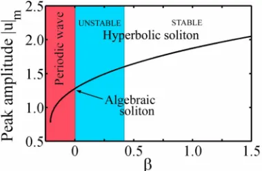
[image:5.595.119.430.74.207.2] [image:5.595.109.505.305.490.2]

[image:6.595.119.309.72.196.2]

Figure 2. (Colour online) Peak amplitude |u|m of solution (3) as a function of  for  = 1.4 (within the conditionally stable regime, as discussed in section 4).  > 0 corresponds to hy-perbolic soliton (3), and  = 0 to algebraic soliton (4). The hyperbolic soliton is unstable against small perturbations when 0 <  <  min  0.42 (blue shaded area). The domain  < 0 (red shaded area) is accessed through analytic continuation, where one finds a transversely-periodic wave. Other parameters:  =  = 1.









2 2 2

2

1 2

2

a   

 _

  

 _ _ 

 

. (4c)

Solution (4) is determined uniquely for any choice of material parameters (,,); its amplitude profile is classified as “Lorentzian” when  = 1, “sub-Lorentzian” when  < 1, and “super-Lorentzian” when 

> 1. The algebraic bright soliton (4) is weakly localized, with relatively slow power-law asymptotics, |u(,)| ~ | + V|–2/ as | + V|  . The beam becomes more localized as  decreases, and such nar-rowing is off-set by an increase in the peak amplitude. This relationship follows directly from the na-ture of a solitary wave: any increase in diffraction must be balanced by an increase in self-focusing.

Theoretical modelling is ultimately concerned with physical phenomena in the laboratory [i.e., the (x,z)] frame. To this end, it is desirable to be able to move easily from scaled to unscaled quantities and coordinates. Such transformations between Helmholtz equations (1) and (2) are fully self-consistent – i.e., exact in their handling of the phase and propagation angle of the beam – since the generality of the (in-plane) Laplacian, 2

zz xx

     , is maintained. In contrast, such transformations can be hindered by the SVEA, where the longitudinal phase shift is always implicitly approximated.

In the (x,z) frame, the longitudinal phase shift  accrued by the hyperbolic soliton (3) during propagation from z = z1 to z = z2 is





1 2

0 0cos 1 4

k n z

  

    , (5)

where  z z₂z₁. When  0, one has that ~k n_{0 0}cosz, and the phase shift is then identical to that picked up by a plane wave propagating in a purely-linear medium with refractive index n0. It is in this sense that algebraic solitons have been interpreted as the threshold for linear wave propagation (i.e., where the carrier wave of the soliton doesn’t ‘see’ the nonlinearity) [17]. The relationship be-tween algebraic soliton (4) and the linear-wave threshold clearly involves the phase in the laboratory reference frame, so an exact transition from hyperbolic to algebraic solutions, valid across the entire range of propagation angles, requires a Helmholtz description.

[image:7.595.118.457.72.185.2]

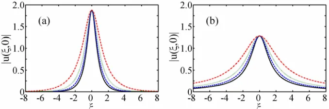
Figure 3. (Colour online) Angular beam broadening effect. (a) Hyperbolic soliton (3) with = 1. (b) Algebraic bright soliton (4), obtained in the limit that   0. Solid line (black):  = 0 (the paraxial profile); dashed line (blue): || = 30; dotted line (green): || = 45; dot-dash line (red): || = 60 (where the beam width appears to have doubled, relative to its on-axis value). Other parameters:  = 1.4 and  =  = 1.





1

2

2

, cos 2 1

1 2

1 4

exp i exp i ,

2 2 1 2 p p V u A V V V                     _           _{  }     _{  } _{ }   _  _ _ _          (6)

where Ap  (1 – ||/||max)1/2, ||max (1 + )(2/)/(2 + )2 and p [–(2 + )||/]1/. This solution exists provided 0 < || < ||max. Propagation (as opposed to evanescence) of the periodic wave requires || < 1/4. This condition places a physical limit on the smallest transverse period of nonlinear wavetrains in relation to the optical wavelength; such considerations are absent from paraxial theory [17]. In parameter regimes of interest, for example,  = 1,   O(1),  = O(1) and  << O(1), one finds that the first of these two conditions is nearly always satisfied before the second comes into play (we also note that the second inequality has no analogue in paraxial theory). The connection between hy-perbolic, algebraic, and periodic waves is illustrated in figure 2.

3.3. Spatial symmetry properties

The symmetry between a forward beam and its backward counterpart can be made explicit by combin-ing the two beams into a scombin-ingle solution. The trigonometric relations cos = 1/(1 + 2V2)1/2 and sin = (2)1/2V/(1 + 2V2)1/2 allow one to eliminate V so that the hyperbolic soliton (3) can be written as





1

, cosh 2 cos sin 1

2

1 4

exp i sin cos exp i .

2 2 2

h h u A                                                   _{ }  _{ } _      

(7a)

In a similar way, the algebraic soliton (4) becomes





1 2 2

, cos sin 1

2

1

exp i sin cos exp i . 2 2 2 a u a                    _{ }     _  _              _{ }  _{ } _      

The propagation angle appearing in solutions (7a) and (7b) now satisfies 180   180, while the remaining parameters are unchanged. One can also re-express the pair of periodic solutions (6) in this type of symmetric form.

Oblique evolution is a potentially dominant Helmholtz contribution since the beam broadening fac-tor (1 + 2V2)1/2 = sec is unbounded: it may be of any order irrespective of  and the system nonlinear-ity. For example, the moderate angle || = 60 implies that 2V2 = 3, and an observer in the (x,z) frame thus perceives the beam width to have doubled relative to its on-axis value (see figure 3). As ||

90, one has that 2V2   and the beam appears to be infinitely broad when viewed from the (x,z) frame (where propagation takes place perpendicularly to the reference direction). This geometrical property of Helmholtz solutions appears in the delocalized wave (6) as an increase in the spatial period , where  = (1 + 2V2)1/20 and 0≡ 2/[(2)

1/2

]. Off-axis effects alone can thus define a scenario in which the angular nonparaxial correction can assume any order 02V2  (equivalent to 0 < ||

90

 ) while the narrowbeam inequality  2 << O(1) is always fully satisfied.

3.4. Conservation laws

Using quite general field-theoretic techniques [33], one can derive three conserved quantities associated with equation (2) that represent the energy-flow, momentum, and Hamiltonian, respectively:

*

2 *

i u u

W d u  u u

      _{ }     _  _       



, (8a)

* * *

* i 2

u u u u u u

M d u u 

                    _  _ _  _             



, (8b)

 

2 2 1

* *

1 2

1

2 1 1

u u

u u u u

H d                  _{   }                 



, (8c)

By writing solution (3) as u(,) = F(s)exp[i(,)], where F is the (real) amplitude distribution and s ( + V)/(1 + 2V2)1/2, the integrals in equations (8a)–(8c) can be expressed more compactly:





1 2 1 4

W     P, (9a)





2 1 4 2

1 2

V

M P Q

V

  

 _   _



, (9b)





2

1 1

1 4 2

2 _{1 2} 2

W

H P Q

V    _      _{  }   _   

. (9c)

The quantities P and Q are given by

 

 

2 2 2 0 2 cosh 1 2 h h

P ds F s  dy A y 

          _ _ _  _  





, (9d)

 

 

 

 

2 2 2

2 2 2

0

2 2 hAh sinh _hcosh 1

d

Q ds F s dy y A y

ds               _{ }  _ _ _  _   _{ }













2 1 2

2

2 2 1

aa

Q   

  

   

 _ _

  

 

, (10b)

where  denotes the Gamma function and 0 <  < 4. Interestingly, Helmholtz bright solitons are also found to satisfy the free-particle relationship H M _VH _VM V , where    _V V. Aside from their physical importance, the integrals in equations (8) allow one to monitor the integrity of the algo-rithm used to solve equation (2) numerically [34].

3.5. The paraxial limit

The corresponding paraxial model [13,17] can be obtained from equation (2) by invoking the SVEA, whereby the operator  is neglected. It is therefore intuitive that when  0, all Helmholtz

con-tributions to beam evolution are negligible, and one should uncover the predictions of paraxial theory. This type of recovery procedure is more subtle than simply setting  = 0. Instead, one is obliged to consider a simultaneous multiple limit [35].

To recover the paraxial solution of Micallef et al [17] from hyperbolic soliton (3), one must allow 0

 (broad beam),  0 (moderate nonlinear phase shift), and V20 (negligible propagation angle). We first consider the asymptotic behaviour of the forward solutions, where  0 . When ap-plied to the hyperbolic soliton, the triple limit leads to













2 1

, ~ cosh 2 1 exp i i

2

h h

V

u A V V



   _    _     _ _

   

 

. (11a)

The  parameter can thus be identified with the on-axis longitudinal phase shift in the corresponding paraxial solution. A similar convergence of the Helmholtz algebraic soliton (4) to its paraxial counter-part requires 0 and V20, so that









2 1

2 2

, ~ 1 exp i i

2

a

V

u a V V



        _   _

  _{ }. (11b)

By applying the multiple limit to the conserved quantities in equations (9), one obtains the familiar par-axial invariants W~P, M ~VP and 1 2

2 ~

H V PPQ for the hyperbolic soliton (the algebraic so-lution requires   0 in the expression for H) [31]. For the backward beams, where ||180, appli-cation of the same multiple limit yields













2 1

, ~ cosh 2 1 exp i i exp i2

2 2

h h

V

u A V V

 _                 _{ }                _{ }      

(11c)

and









2 1 2 2

, ~ 1 exp i i exp i2

2 2

a

V

u a V V

 _            _{ }  _{ }  _{   }       _{ }  

[image:10.595.111.451.73.184.2]

Figure 4. (Colour online) Stability characteristics of hyperbolic solitons. (a) Variation of the beam power P with  [solid line (black):  = 0.9; dashed line (blue):  = 1.0; dotted line (green):  = 1.2; dot-dash line (red):  = 1.4]. For 0 <   1, the solutions are uncondition-ally stable (dP/d > 0 for all   0). For 1 <  < 2, the solutions are conditionally stable, so that dP/d > 0 only when  > min(). (b) The boundary between stable and unstable solutions in the (, ) plane is determined (numerically) by the curve min().

respectively, while the invariants become W ~P, M ~VP, and 1 2 2

~ 3

H V P PQP . Since the latter set of results retain -dependent contributions, it is clear that backward fields have no ana-logue in paraxial theory. This confirms the fact that paraxial models can support wave propagation in a single longitudinal direction only.

4. Stability of Helmholtz bright solitons

Linear analysis has predicted that plane-wave solutions to NLH equations with arbitrary dispersive nonlinearity functions are modulationally stable in the same parameter regions as their paraxial coun-terparts [36]. However, the stability of localized solutions against arbitrary perturbations is a much more interesting problem: such stability is a key property of solitons. Without loss of generality, we set

 =  = 1 throughout this section.

4.1. Analysis

The stability of paraxial bright solitons (11a) has been studied by Micallef et al [17] using the well-known Vakhitov-Kolokolov (VK) criterion [30,37]. Spatial symmetry allows the same criterion to pre-dict the stability properties of Helmholtz solitons [36,38]. This is because an isolated off-axis beam can always be observed from the “on-axis” frame of reference by means of a rotation of the coordinate axes. In the on-axis frame, where V = V2 = 0, beams with  << O(1) and  << O(1) are quasi-paraxial since the forward solution (3) exhibits only an O() correction to the longitudinal phase shift.

The VK criterion states that bright solitons can be stable against small perturbations if dP/d > 0, where



;





, ; ;



2

P   d u    







_

(12)

[we note, in passing, that equations (12) and (9d) are formally identical for paraxial solitons]. Satisfac-tion of the VK criterion is a necessary but not sufficient condiSatisfac-tion for stability [36]; simulaSatisfac-tions are es-sential to establish the robustness of solutions against arbitrarily-large perturbations. Hyperbolic soli-tons are predicted to be unconditionally stable when 0 <   1 since, for that range of , the VK ine-quality dP/d > 0 is satisfied for any   0. However, figure 4(a) reveals that when 1 <  < 2, the slope dP/d > 0 only when  exceeds a minimum value, denoted by min. Regions of stability in the (,

[image:11.595.110.449.68.298.2]

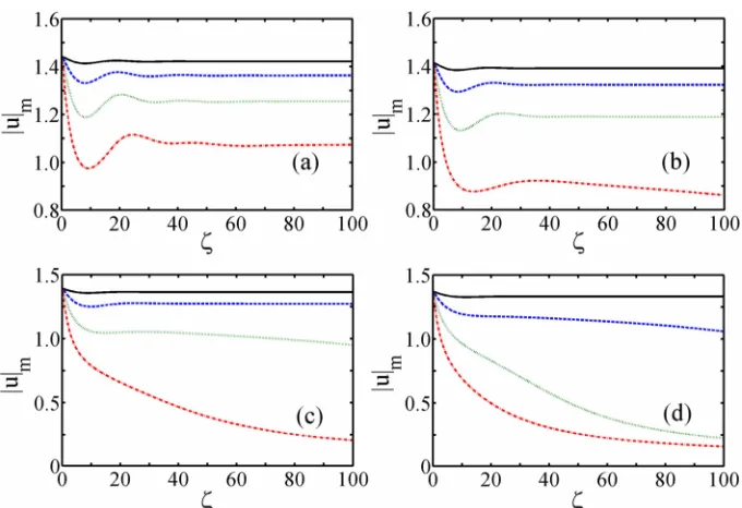
Figure 5. (Colour online) Evolution of the peak amplitude |u|m of a perturbed hyperbolic soli-ton with  = 1 when (a)  = 0.5, (b)  = 0.6, (c)  = 0.7 and (d)  = 0.8. Solid lines (black): || = 10; dashed lines (blue): || = 20; dotted lines (green): || = 30; dot-dash lines (red): || =

40.

4.2. Hyperbolic solitons

The stability of hyperbolic solitons is considered through the perturbed input beam



, 0



cosh



2



1 1 exp i 1 4 ₂ 1 2

h h

u A V

V

 _

     



 _{  }

 

  _ _

 

  _

 

, (13)

whose launching angle is  = tan–1[(2)1/2V]. By applying a rotational transformation [39], one can see that the initial condition (13) is equivalent to an on-axis Helmholtz soliton whose width has been re-duced by a factor of (1 + 2V2)1/2 = sec . For  = 10–3 ( = 10–4), launching angles of || = 10, 20,

30 and 40 correspond to transverse velocities of |V|  3.94, 8.14, 12.91 and 18.76 (|V|  12.47, 25.74, 40.82 and 59.33), respectively. These angles are clearly non-trivial and lie outside the scope of paraxial theory.

In the unconditionally stable domain (0 <   1), evolution is generally characterized by mono-tonically-decreasing oscillations in the beam parameters (amplitude, width, and area = ampli-tudewidth). These oscillations are accompanied by a small amount of radiation, and they disappear as

   to leave a stationary state (see figure 5). Solitons with 0 <   1 can thus generally be inter-preted as stable fixed-point attractors: the emission of radiation throughout reshaping provides a mechanism for local dissipation while the system remains globally conservative [36,38]. As discussed in the preceding subsection, there should be no instability in the range 0 <   1 (as prescribed by the VK inequality). However, simulations have revealed that as   1, sufficiently large perturbations can induce a diffractive instability whereby the amplitude of the beam tends to zero as   .

To gain insight into the propagation properties of conditionally-stable hyperbolic solitons (where 1 <  < 2), it is instructive to recognize that the power Pin(,;V) of the perturbed input beam (13) is re-lated to the power P(,) of the unperturbed beam by













in ₂

,

, ; , cos

1 2

P

P V P

V

 

    



 



[image:12.595.110.448.72.183.2]

Figure 6. (Colour online) (a) Beam power calculated from equation (12) for hyperbolic soliton (3) with  = 1.4, where (min, Pmin)  (0.42, 3.46). The criterion dP/d > 0 is met when  >

min (unshaded region). (b) Theoretical prediction from equation (15) for the maximum launch-ing angle of input beam (13) before the onset of instability, where Pin Pmin.

Figure 7. (Colour online) Long-lived self-persistent reshaping oscillations in the peak ampli-tude |u|m of a perturbed (conditionally-stable) hyperbolic soliton (3) with  = 1.4. For  = 1, equation (15) predicts that ||max 10.7. Instability sets in when |θ| is slightly less than the theoretical value of ||max.

where P is given by equation (12). That is, || > 0 decreases the power of the input beam relative to its unperturbed value (i.e., relative to the power of the exact solution with the same parameters). Figure 4(a) suggests there is a minimum power Pmin that can sustain a propagating soliton; when Pin < Pmin, one expects that no stationary states exist and that the input beam will transform into radiation modes [30]. Thus, (min, Pmin) are the coordinates of the local minimum in the P() curve [see figure 6(a)]. One can then expect to encounter a maximum perturbation, against which the soliton is stable, through the fol-lowing condition: Pin = Pmin when || = ||max. It can then be shown that for any input beam with  >

min,





1 2 2

max

min

tan P 1

P



_{ } 

 

 _{ } 

_{ } 

 

. (15)

[image:12.595.110.292.267.389.2]

[image:13.595.109.449.68.301.2]

Figure 8. (Colour online) Evolution of the peak amplitude |u|m of a perturbed algebraic bright soliton when (a)  = 0.5, (b)  = 0.6, (c)  = 0.7 and (d)  = 0.8. Solid lines: || = 10; dashed lines: || = 20; dotted lines: || = 30; dot-dash lines: || = 40.

finds that the evolving soliton diffracts toward a zero-amplitude state (see figure 7).

4.3. Algebraic solitons

Analysing the stability of algebraic solitons is a notoriously difficult task. Conventional nonlinear-perturbative techniques tend to become frustrated in all but the simplest cases because of their relatively slow asymptotics (i.e., power-law instead of exponential) [30]. Some insight can be gained from in-spection of figure 4(a). For example, in the region where the hyperbolic solutions are unconditionally stable (0 <   1), the beam power has a positive slope (i.e., dP/d > 0) at  = 0. However, when  > 1, one finds that dP/d < 0 at  = 0. Thus, algebraic solitons are expected to be always unstable when

 > 1. Micallef et al [17] suggested that paraxial algebraic solitons (11b) are inherently unstable due to the absence of an arbitrary internal parameter. Their simulations confirmed that, even when 0 <   1, algebraic solitons are weakly unstable. Pelinovsky et al attributed this instability to resonant interac-tions with infinitely long linear waves [30].

We now undertake a fully nonlinear (i.e., numerical) stability analysis of Helmholtz algebraic soli-tons through consideration of the input beam







2 2



1

2

, 0 1 exp i

1 2

a

V

u a

V



   



  

   

 



 

. (16)

[image:14.595.111.449.72.183.2]

Figure 9. (Colour online) Comparison of the angular beam broadening effect for the algebraic dark soliton (17) [(a)] with that of the corresponding (i.e.,  = 2) bright soliton (4) [(b)]. As 

 , one finds that the dark solution behaves as u ~ /a (reflecting the  phase shift). Solid line (black):  = 0 (the paraxial profile); dashed line (blue): || = 30; dotted line (green): || = 45; dot-dashed line (red): || = 60. Other parameters:  =  = 1.

5. Helmholtz algebraic dark solitons

5.1. Exact analytical solutions

Equation (2) permits the existence of algebraic dark solitons in the particular case of a cubic-quintic nonlinearity (i.e., when  = 2). In symmetric form,





1 2 2

2

, cos sin cos sin 1

2 2

1 4

exp i sin cos exp i ,

2 2 2

u        a    

 

  

  

  



 

   

 

 _  _{ }  _ 

 

 _   _

     

      

 

 

 

(17)

where a2  2/6,   (3/)1/2a2 and   –2/4. Like its bright counterpart [solution (4)], the dark solution is specified uniquely by the choice of  and . There is a phase shift of  radians across the transverse extent of the field, and an absolute-zero in the field at the beam centre (see figure 9). How-ever, the solution is structurally distinct from the more familiar phase-topological dark solitons [40,41]. In passing, we note an asymmetry between algebraic solutions (17) and (4) [in the case of  = 2] – while the intensity profiles of canonical bright and black Kerr solitons, Ib = sech2(s) and Id = tanh2(s), are related by Id = 1 – Ib, the same type of relationship does not hold for bright and dark algebraic beams.

One can now consider the multiple limit 0, 0 and V20. From the forward solu-tion, one can recover the paraxial soliton of Hayata and Koshiba [13], namely













2 1 2

2 2

, ~ 1 exp i i

2

V

u     V a  V V  

    

 

 _   _   _  _ 

   

 

. (18a)

The backward solution tends to













2 1 2

2 2

, ~ 1 exp i i exp i2

2 2

V

u     V a  V V   



     _{ }

 

     _  _  _ _

  _{     }

 

, (18b)

[image:15.595.118.301.73.194.2]

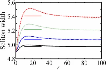
Figure 10. (Colour online) Evolution of the beam full-width of a perturbed algebraic dark soliton. The width tends asymptotically toward the value _~ (1+2V2)1/20, where 0 2/a (horizontal bars). Solid line (black): || = 10; dashed line (blue): || = 15; dotted line (green): || = 20; dot-dash line (red): || = 25. The widths have been calculated by fitting the numerical data to the nonlinear refractive-index function nNL = –|u|2 + |u|4 in combina-tion with solucombina-tion (17). For larger values of ||, the evolving beam radiates more strongly and suffers fluctuations to its shape that can complicate interpolation. Other parameters:  =  = 1.

5.2. Numerical stability analysis

The apparent absence of a suitable stability criterion has so far rendered an in-depth analysis of solution (17) problematic. For instance, one cannot apply the renormalized-momentum integral [42] since there is no intrinsic-velocity parameter [41]. One also encounters divergences in the integral conserved quan-tities [equations (8a)–(8c)] because the solution does not break up in the way the renormalization method demands (i.e., a plane-wave background modulated by an obliquely-propagating grey “dip”).

Here, we investigate the stability properties of Helmholtz algebraic dark solitons numerically using the input beam







2 2



1 2

2

1 4

, 0 1 exp i

1 2

u a V

V



   



  _ 

  _ _



 

. (19)

This initial condition corresponds to launching an exact paraxial soliton (that does not account for the beam-broadening factor). The full width of the beam is found to tend towards an asymptotic value



 = (2/a)(1+2V2)1/2 as   , eventually leaving a stationary beam (see figure 10). Simulations show that the dark beam can be robust against perturbations, even through its bright counterpart [solu-tion (4) with  = 2] is always unstable. Thus, one can interpret the dark solitons as fixed-point attrac-tors. Similar qualitative behaviour has been uncovered in the propagation properties of Helmholtz Kerr dark solitons [41].

6. Conclusions

stable-attractor properties when subject to large angular perturbations. Numerical analysis has also provided evidence of algebraic dark-soliton stability.

The new solitons reported here have innate mathematical appeal as exact solutions to generic non-integrable elliptic equations. Our results are also of physical interest, particularly in photonics, where we propose that Helmholtz soliton theory will play a central role in the design of future integrated-optic devices that exploit non-trivial angular geometries. Indeed, the coexistence of many different solution families (plane waves, hyperbolic and algebraic solitons) could open up the possibility of exciting new multiplexing [21] and interface [22] applications within Helmholtz-nonparaxial configurations.

References

[1] Dodd R K, Eilbeck J C, Gibbon J D and Morris H C 1982 Solitons and Nonlinear Wave Equa-tions (London: Academic Press)

Remoissenet M 1999 Waves Called Solitons: Concepts and Experiments, 3rd Ed (Berlin: Springer-Verlag)

Infeld E and Rowlands G 2000 Nonlinear Waves, Solitons and Chaos, 2nd Ed (Cambridge: C.U.P.)

[2] Kivshar Y S and Malomed B A 1989 Rev. Mod. Phys.61 763

[3] Klaus M, Pelinovsky D E and Rothos V M 2006 J. Nonlinear Sci. 16 1 Ablowitz M J and Satsuma J 1977 J. Math. Phys.19 2180

[4] Pelinovsky D E and Grimshaw R H J 1997 Phys. Lett. A 229 165 Ono H 1976 J. Phys. Soc. Japan41 1817

[5] Brunhuber C, Mertens F G and GaidideiY 2007 Eur. Phys. J B 57 57 [6] Fokas A S, Pelinovsky D E and Sulem C 2001 Physica D 152 189

Satsuma J and Ablowitz M J 1979 J. Math. Phys.20 1496 Watanabe Y and Tajiri M 1998 J. Math. Phys.67 705

Tajiri M, Arai T and Watanabe Y 1998 J. Phys. Soc. Japan67 4051 [7] Pelinovsky D E and Sulem C 1998 J. Math. Phys. 39 6551

Benjamin T B 1966 J. Fluid Mech. 25 241 Ono H 1975 J. Phys. Soc. Japan39 1082

Meiss J D and Pereira N R 1978 Phys. Fluids21 700

[8] Kennel C F, Buti B, Hada T and Pellat R.1988 Phys. Fluids31 1949

[9] Manakov S V, Zakharov V E, Bordag L A, Its A R, and Matveev V B 1977 Phys. Lett. A 63 205 [10] Skryabin D V and Yulin A V 2006 Phys. Rev. E 74 046616

[11] Belenov E M and Poluéktov 1969 Sov. Phys. JETP28 754 Hanamura E 1974 J. Phys. Soc. Jap.37 1598

[12] Mihalache D, Truta N, Panoiu N C, and Baboiu D M 1993 Phys. Rev. A 47 3190 Mihalache D and Panoiu N C 1993 J. Phys. A: Math. Gen. 26, 2679

[13] Hayata K and Koshiba M 1995 Phys Rev. E 51 1499 Hayata K and Koshiba M 1995 Opt. Lett. 20 1131

[14] Hayata K and Koshiba M 1994 J. Opt. Soc. Am. B 11 2581 Hayata K and Koshiba M 1995 Phys. Rev. E 51 5155

[15] Alatas H, Iskandar A A, Tjia M O and Valkering T P 2006 Phys. Rev. E 73 066606 Grimshaw R and Malomed B 1994 Phys. Rev. Lett. 72 949

[16] t’Hooft G 1976 Phys. Rev Lett. 37 8 Polyakov A M 1974 JETP Lett.20 194

[17] Micallef R W, Afansjev V V, Kivshar Y S and Love J D 1996 Phys. Rev. E 54 2936 [18] Kivshar Y S 1998 Opt. Quant. Electron. 30 571

Kivshar Y S and Luther-Davies B 1998 Phys. Rep.298 81 Stegeman G and Segev M 1999 Science286 1518

[19] Zakharov V E and Shabat A B 1972 Sov. Phys. JETP 34 62 Satsuma J and Yajima N 1974 Suppl. Prog. Theor. Phys. 55 284 Gordon J P 1983 Opt. Lett. 8 596

Cohen O, Uzdin R, Carmon T, Fleischer J W, Segev M and Odouov S 2002 Phys. Rev. Lett. 89

Sheppard A P and Haelterman M 1998 Opt. Lett. 23 1820 Fibich G 1996 Phys. Rev. Lett.76 4356

[25] Lax M, Louisell W H and. McKnight W B 1975 Phys. Rev. A 11 1365 [26] Chi S and Guo Q 1995 Opt. Lett. 20 1598

[27] Ciattoni A, Crosignani B, Di Porto P, Scheuer J and Yariv A 2006 Opt. Exp.14 5517 Ciattoni A, Crosignani B, Mookherjea S and Yariv A 2005 Opt. Lett.30 516

Crosignani B, Yariv A and Mookherjea S 2004 Opt. Lett. 29 1524

Ciattoni A, Di Porto P, Crosignani B and Yariv A 2000 J. Opt. Soc. Am. B 17 809

[28] Mihalache D, Bertolotti M and Sibilia C 1989 Progress in Optics ed. E. Wolf (Amsterdam: El-sevier) 27 229

Snyder A W and Mitchell D J 1993 Opt. Lett.18 101

[29] Pushkarov K I, Pushkarov D I and Tomov I V 1979 Opt. Quantum Electron.11 471 Pushkarov K I and Pushkarov D I 1980 Rep. Math. Phys.17 37

[30] Pelinovsky D E, Afanasjev V V and Kivshar Y 1996 Phys. Rev. E 53 1940 [31] Akhmediev N, Ankiewicz A and Grimshaw R 1999 Phys. Rev. E 59 6088 [32] Biswas A 2004 Opt. Commun.235 183

[33] Goldstein H 1982 Classical Mechanics 2nd Ed. (Addison Wesley)

[34] Chamorro-Posada P, McDonald G S and New G H C 2001 Opt. Commun.192 1 [35] Chamorro-Posada P, McDonald G S and New GHC 1998 J. Mod. Opt.45 1111

[36] Christian J M, McDonald G S and Chamorro-Posada P 2007 J. Phys. A: Math. Theor.40 1545 Christian J M, McDonald G S and Chamorro-Posada P 2007 J. Phys. A: Math. Theor. 40 8601

Corrigendum

[37] Vakhitov M G and Kolokolov A A 1973, Radiophys. Quantum Electron. 16 783 Laedke E W, Spatschek K H and Stenflo L 1983 J. Math. Phys.24 2764

[38] Christian J M, McDonald G S and Chamorro-Posada P 2007 Phys. Rev. A 76 033833 Christian J M, McDonald G S and Chamorro-Posada P 2007 Phys. Rev. A 76 033834 Christian J M, McDonald G S and Chamorro-Posada P 2007 Phys. Rev. A 76 049905(E) [39] Chamorro-Posada P, McDonald G S and New G H C 2000 J. Mod. Opt.47 1877

[40] Zakharov V E and Shabat A B 1973 Sov. Phys. JETP 37 823 [41] Chamorro-Posada P and McDonald G S 2003 Opt. Lett.28 825

[42] Pelinovsky D E, Kivshar Y S and Afansjev V V 1996 Phys. Rev. E 54 2015 Barashenkov I V 1996 Phys. Rev. Lett.77 1193