Multi scale Gaussian Segmentation via Graph Cuts

2017 International Conference on Computer Science and Application Engineering (CSAE 2017) ISBN: 978-1-60595-505-6

Multi-scale Gaussian Segmentation via Graph Cuts

Ye Zhang* and Kun He

College of Software, Jiang'an campus of Sichuan University, 610225 Chengdu, China

ABSTRACT

Towards the improvement of image segmentation performance, a new improved segmentation method is proposed which combines the use of multi-scale information. The multi-scale information of an image, generated by a linear Gaussian smoothing function through an interactive scheme that provides different levels of image cues which help to capture the abundant content of the image. However, Gaussian smoothing cannot generate an optimum solution to the specific scale level. According to the boundaries sensibility to scale, a convergence constraint based on the significant scale level of the segmented regions is constructed. The experimental results show that this method has superior advantages in performance and towards noise images.

INTRODUCTION

Image segmentation is a process of subdividing an image into several sub-regions based on contents. Effective segmentation technologies provide image retrieval and object analyzing with useful information [1]. They have been widely used in fields like medical analysis [2] and object localization [3].

There are many segmentation technologies based on graph theory, such as N-cuts [4], Grab cuts [5] and Graph Cuts [6] [7] [8] [9]. The segmented regions using N-cuts have no semantic concept for only exploiting low-level nature information. With the help of user interaction [10], Grab Cuts and Graph Cuts extract semantic objects combining boundary and regional information. In Grab Cuts, regional energy function has locality because of regional Gaussian fitting. It leads to local optimum of the segmentation results. Graph Cuts uses histograms to obtain global information, which improves the segmentation performance incomparison with Grab Cuts. However, both cannot produce correct segmentation results on noisy images or images with overlap appearance between objects and background owing to taking given-scale information into account [11]. The full convolution nets [12] which exploits different-scale information, is proposed to implement semantic image segmentation. However, it needs massive image data which is accurate to pixel level [13] for deep learning.

RELATED WORK ON MULTI-SCALE INFORMATION

Image segmentation exploiting single-scale information cannot produce correct results. In order to improve the segmentation performance, we use Gaussian smoothing to obtain multi-scale information. Let I0 denotes the luminance component of a color image and G_ is the Gaussian function [15]. Smoothing component I is given by

0

*

I I G_ (1)

where  is the standard deviation of Gaussian and decides the smoothing scales. With

 increasing, the small-scale objects of an image are smeared to large structures step by step. It is difficult to get an appropriate  without prior knowledge. To optimize , we use iteration to produce a series of components Ik using Gaussian kernel

0,1, , ,

k

G k  k according to equation 1. To reduce computation cost, according

to the Gaussian sequential convolution, that is 2 2 2 0

     , the different-scale smoothing component Ik can be obtained based on the last smoothing component

1

k

I  , instead of original image I0, just as follows:

0

0 1 k

I     I   I  (2)

where ₀ is the original standard deviation of Gaussian applied to original image 0 I

and  is applied directly to the last smoothing component.

At step k , smoothing component Ik only depends on Ik1, leading that the small-scale objects are smeared step by step, the appearance of _Ik _{is more tight}

cohesion than that of Ik-1, the histograms of components appear peak distribution (the second column in Figure 1). If smoothing scale increases continuously, the distribution of histogram is almost invariant but edges are blurred (the bottom-left corner sub-image in Figure 1).

PROPOSED SEGMENTATION MODEL

Graph Cuts can get global optimum for image segmentation. We exploit it to segment the smoothing component k

I . The segmentation can be estimated as a global minimum by standard Minimum Cut algorithm [16]:

( k) ( k) ( k)

E I  R I B I (3)

where R I( k) donates regional information, which is

1

( ) = ( ) N

k k

p i i

R I R I





Here ( k) p i

R I represents the individual penalties for assigning pixel i to "object"

2

( , )

( ) exp( || ( ) || )

( , )

k k k

p q p q G

B I I I

dist p q 







where G represents the set of all the neighboring pixels pairs and dist p q( , ) is the Euclidean distance between pixels p and q. The  should be calculated to switch appropriately between high and low contrast edge, that is

-1 2

0.5 (Ik_p I_qk)

    (6)

where term  is expectation over the smoothing component Ik.

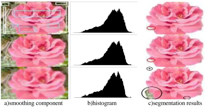
The multi-scale information is obtained by linear Gaussian kernel, leading that there is not a solution to the scale optimum problem. An image from the international web was smoothed with different number of iterations. Part results are shown in Figure 1. With smoothing scale increasing, performance in high-scale segmentation is superior to that in low-scale segmentation (seen the red oval in the first and second row). When the number of iteration keeps on increasing, improper-scale information causes decrease of the segmentation performance (seen the blue oval in the third row).

a)smoothing component b)histogram c)segmentation results

Figure 1. The smoothing components, histograms, and segmentation results. From top to bottom, 0,2,10 iterations are performed. The x- and y-axis of the histogram are pixels and frequency, respectively. The blue and white rectangles on the original image are objects and background user selected, respectively.

In order to evaluate segmentation performance, we construct a convergence condition based on the significant level of segmentation sub-regions on adjacent scale components. It is defined as follows:

1 1

1

( )

( , )

max{ ( ), ( )} k k

k k

k k

card S S C S S

card S card S

 





 (7)

where C S S( k, k1) represents the significant level of segmentation performance on two

adjacent scale component k

I and k 1

I  . k

S represents the set of pixels which belong to object regions in the segmentation result when segmenting the smoothing component

k

segmentation performance between two adjacent scale components decrease,

-1

( k, k )

C S S will increase. With scale increasing, the appearance has more peak distribution, leading that the significant level of the segmentation increases monotonically. If the iteration number tends to infinitely great, regional diversity disappears, which causes the significant level to monotonously decrease. When the confidence level satisfies the following condition, the smooth scale is terminated (see Figure 2):

-1 1 -2

( k, k ) ( k , k ) 0

C S S C S  S  (8)

Algorithm1: Procedural steps of the proposed method

Initialized parameters - 0 0

0

, , , , ,

I  S  .

Begin

Selecting region of interest and background regions and Initializing S0

Do for each kscale [do … while loop]

Applying Gaussian smoothing through the equation 2

Substitute in Gaussian component Ik into equation 3

While (Until convergence is reached) given by equation 8 Save output results and computation times.

End

Figure 2. Procedural steps of the proposed method.

EXPERIMENTAL RESULTS

The experiments were conducted according to algorithm1 using C language in VC6.0 on the PC with Duo Core i5 CPU @2.0GHZ and 4GB of RAM. During the experiment,  in equation 5 was set to 50 and since the edge boundary and region information is equally important,  was set to 4.0 in equation 3. Images were segmented using the Graph Cuts on multi-scale smoothing components and the parameters 0 and  decide the smoothing scale. To analyze the relationship between

these two parameters and the segmentation performance, an image in Berkeley segmentation database (https://www2.eecs.berkeley.edu/Research/Projects/ CS/ vision/

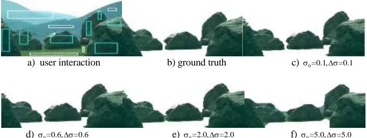
bsds/BSDS300/html/dataset/images/color/test-026-050.html) was smoothed with different ₀ and , and partial results are shown in Figure 3. Ground truth represents the correct segmentation result. As we can see, with smoothing scale increasing, segmentation performance is getting better first and then getting worse. In the following experiments, ₀ and  were set to 0.6 by optimizing performance against ground truth over 15 images.

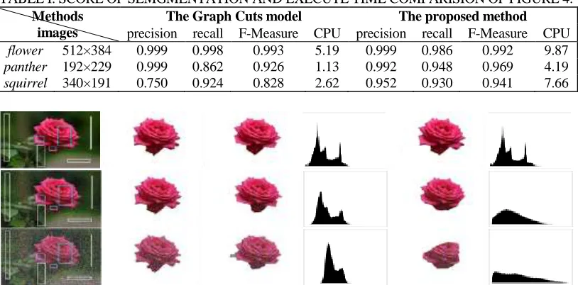
performance using proposed method is almost the same as that using Graph Cuts model. The effect of the proposed method on images in which there is a wide range of luminance in object region, is better than that of the Graph Cuts (the red oval in row 2). For images with overlap appearance between objects and background, in comparison with Graph Cuts, the proposed method is out-performance (the last row) because the appearance of the multi-scale component have more peak distributions. However, as we can see in TABLE I, the proposed method is computationally longer than the Graph Cuts.

Noise is one of the factors causing poor segmentation performance. In order to test robustness against noise using these two methods, we conduct experiments on images with additive Gaussian noise. Partial results are shown in Figure 5. The scores of segmentation on images with and without noise are listed in TABLE II. For original image, the performance of both methods is almost the same. The appearance distribution of the noisy image causes the negative effects on segmentation performance using Graph Cuts model. The segmentation results using the proposed method are out-performance compared to those using the Graph Cuts because multi-scale smoothing ameliorate the appearance distribution of the noisy images (the fourth and sixth column). Although the proposed method is insensitive to noise, the CPU time is longer than Graph Cuts. The lower the PSNR, the longer the CPU time.

a) user interaction b) ground truth c) 0=0.1,=0.1

d) 0=0.6,=0.6 e) 0=2.0,=2.0 f) 0=5.0,=5.0

Figure 3. Segmentation results with different parameters ₀ and .

a) user interaction b) ground truth c) proposed method d) Graph Cuts

TABLE I. SCORE OF SEMGMENTATION AND EXECUTE TIME COMPARISION OF FIGURE 4.

Methods images

The Graph Cuts model The proposed method

precision recall F-Measure CPU precision recall F-Measure CPU

flower 512×384 0.999 0.998 0.993 5.19 0.999 0.986 0.992 9.87

panther 192×229 0.999 0.862 0.926 1.13 0.992 0.948 0.969 4.19

squirrel 340×191 0.750 0.924 0.828 2.62 0.952 0.930 0.941 7.66

Figure 5. Comparison of the proposed method with Graph Cuts on real images with noise. Column 1-6, user interaction, ground truth, the proposed method, the histograms of the smoothing component, the Graph Cuts model, and the histograms of the image. Row 1-3: original image, PSNR (Peak Signal

Noise Ratio) = 21.26, PSNR = 14.01.

TABLE II. SCORE OF SEGMENTATION AND CPU TIME COMPARISION OF NOISY IMAGE.

method

PSNR

The Graph cuts model The proposed method

precision recall F-Measure CPU precision recall F-Measure CPU

original

image 0.996 0.999 0.993 3.02 0.995 0.947 0.970 8.44

26.53 0.998 0.974 0.981 3.88 0.987 0.901 0.942 8.26

23.33 0.988 0.907 0.946 5.25 0.994 0.903 0.947 12.58

23.08 0.976 0.909 0.942 6.42 0.996 0.922 0.958 13.18

21.26 0.988 0.908 0.946 9.26 0.985 0.928 0.956 15.60

18.46 0.996 0.714 0.832 11.60 0.993 0.908 0.920 20.51

14.01 0.981 0.611 0.753 16.13 0.975 0.927 0.958 23.37

average 0.989 0.860 0.913 7.93 0.989 0.919 0.950 14.56

CONCLUSIONS

ACKNOWLEDGEMENT

This work was supported by the Sichuan Province Natural Science Foundation of China (2016JZ0014).

REFERENCES

1. Zhang X., Su H., and Yang L., et al. 2015. “Fine-grained histopathological image analysis via robust

segmentation and large-scale retrieval,” Computer Vision and Pattern Recognition IEEE,

29(5):5361-5368.

2. Masood S., Sharif M., and Masood A., et al. 2015. “A survey on medical image segmentation,”

Current Medical Imaging Reviews, 11(1): 3-14.

3. Brejl M. and Sonka M. 2000. “Object localization and border detection criteria design in edge-based

image segmentation: automated learning from examples,” IEEE Transactions on Medical Imaging,

19(10): 973-985.

4. Shi J. and Malik J. 2000. “Normalized cuts and image segmentation,” IEEE Computer Society,

22(8):888-905.

5. Rother C., Kolmogorov V. and Blake A. 2004. “‘GrabCut’: interactive foreground extraction using

iterated graph cuts,” ACM SIGGRAPH,23(3):309-314.

6. Boykov, Y. Y. and M. P. Jolly. 2001. “Interactive Graph Cuts for Optimal Boundary & Region

Segmentation of Objects in N-D Images,” Proc. Int’l Conf. Computer Vision, 1, pp. 105-112.

7. Wang T., Ji Z., and Sun Q., et al. 2016. “Label propagation and higher-order constraint-based

segmentation of fluid-associated regions in retinal SD-OCT images,” Information Sciences, s

358-259(C), 92-111.

8. Wang T., Sun Q., and Ji Z., et al. 2016. “Multi-layer graph constraints for interactive image

segmentation via game theory,” Pattern Recognition, 55(C):28-44.

9. Wang T., Ji Z., and Sun Q., et al. 2016. “Interactive Multilabel Image Segmentation via Robust

Multilayer Graph Constraints,” IEEE Transactions on Multimedia,18(12): 2358-2371.

10. Ning J., Zhang L., Zhang D. and Wu C. 2010. “Interactive image segmentation by maximal similarity

based region merging,” Pattern Recognition, 43(2):445–456.

11. Shi J. and Malik J. 2002. “Normalized cuts and image segmentation,” IEEE Computer Society,

22(8):888-905.

12. Kalinovsky A. and V. Kovalev. 2016. “Lung Image Segmentation Using Deep Learning Methods

and Convolutional Neural Networks,” presented at Xiii International Conference on Pattern Recognition and Information Processing.

13. Long J., Shelhamer E., and Darrell T. 2015. “Fully convolutional networks for semantic

segmentation,” Computer Vision and Pattern Recognition IEEE, 79(10):3431-3440.

14. Zheng S., Yuille A. and Tu Z. 2010. “Detecting object boundaries using low-, mid-, and high-level

information,” IEEE Conference on Computer Vision and Pattern Recognition, 114(10):1-8.

15. Witkin A. P., Baudin M. and R. O. Duda. 1986. “Uniqueness of the Gaussian kernel for scale-space

filtering,” IEEE Transactions on Pattern Analysis and Machine Intelligence, 8(1): 26-33.

16. Boykov Y. and Kolmogorov Y. 2004. “An experimental comparison of min-cut/max-flow

algorithms for energy minimization in vision,” IEEE Transactions on Pattern Analysis and Machine