2017 International Conference on Computer, Electronics and Communication Engineering (CECE 2017) ISBN: 978-1-60595-476-9
Performance Analysis of Accurate Time Delay and Its Influence
on Sonar Beam Formation
Zhi-zhong LI, Zhe CHEN, Zhong-liang XU and Yu-sheng CHENG
China Navy Submarine Academy, Qingdao 266000, ChinaKeywords: Accurate time delay, Sonar beam formation.
Abstract. The time delay accuracy affects the processing performance of the sonar signals. This
paper studies the implementation principles of such accurate time delay methods as linear interpolation method, Sinc function interpolation method, Lagrange interpolation method and Farrow filter method and investigates the performance of different accurate time delay methods by simulation as well as the influence of accurate time delay on beam formation. The research results show the images of accurate time delay will be smoother, and lower in side lobe and less in false peak than that of conventional time delay. But both of them have the same beam width.
Introduction
During the array signal processing, the time delay accuracy of the signals between array elements will directly influence the signal processing performance[1]. The traditional method to realize the time delay of digital signal is to apply digital delay line[2]. This method will bring the system error of half sampling period. In digital sonar system, time delay error reduces signal-to-noise ratio (SNR) formed by sonar beam[3], which affects the passive ranging accuracy of sonar[4], thereby impacting the technical performance of the sonar. To improve time delay accuracy of signals, this paper systematically studies the theory of such fractional time delay methods as linear interpolation method[5,6], Sinc function interpolation method[7,8], Lagrange interpolation method[9,10] and Farrow filter method[11,12], and conducts simulation verification on different fractional time delay methods. The fractional time delay method may be applied to sonar beam formation, sonar array signal simulation system and passive ranging system based on sonar array element time delay estimation, so as to improve the performance of the sonar system[13].
Basic Principle
Conventional Time Delay
The traditional method to realize the time delay of digital signals is to apply digital delay line, by which the digital signals that are discretized after sampling are transmitted to one shift register. The drive period of this shift register is exactly equal to signal sampling period. The length of delay line is equal to the max. delay time required for beam formation and then apply the traditional method (digital delay line) to transmit the digital signals that are discretized after sampling to one shift register for reading them out. Driven by drive signals, the signals are moved forward a bit in each period and then repeated to obtain the delayed time sequence digital signals.
Usually, the delay time nodes will be determined by use of the nearest integer, which is a choice of the nearest neighbor. Supposed we want to delay time, then the specific delay time nodes will be expressed as:
int( / )s
means the rounding calculation which guarantees the compensation error of delay time is distributed in [Ts/ 2,Ts/ 2]. So, the discretized continuous time delay signals in any time domain can be expressed in number as:
( ) ( S S)
x n x nT LT (2)
Accurate Time Delay of Sinc Function
After any time delay is performed for one continuous time signal ( )x t , ( )y t can be obtained as follows:
( ) ( )
y t x t (3) After Fourier transformation, the type of frequency domain is obtained as follows:
( ) ( ) j t j ( )
Y x t edt eX
(4) In an ideal circumstance of the continuous system, we could obtain the transfer function of time delay filter:( ) ( )
( )
j
Y
H e
X
(5)
The formula above is expressed in time domain as:
( ) ( ) sin ( )
h t t c t (6) After the signal is subject to discretization in sampling period Ts of Nyquist sampling theory, the following will be obtained:
+
k=-( ) ( )sinc( )
( )*sinc( )
( )* ( )
y n x k n D k
x n n D
x n h n
(7)
From the inference above, it can be seen that performing time delay for a signal is equivalent to transmitting the signal into a special filter for processing. The filter could be able perform fractional time delay for the signal, bringing the possibility to realize accurate time delay for broad-band signals. It can be understood as using Sinc function sampling value subjected to time delay to perform convolution on the known waveform sampling amplitude value to estimate waveform amplitude value between original sampling values.
Linear Interpolation Time Delay Method
f
t
a b
a
f
b
f
m
f
m
[image:2.612.217.396.579.694.2]1p p
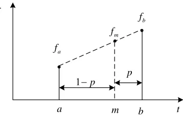
The linear interpolation principle is shown in Figure 1 where m is ideal interpolation point (also called ideal time delay point), a and b refer to two adjacent points of discrete signals respectively.
( )
m a b a
f f f f p kx (8)
Where k is attenuation coefficient for adjustment; to maintain smoothness of signals, it is required thatfm[ , ]fa fb .
The gradient at the point of mis defined as follows:
2 2 2 1 1 am bm m m a
am b a
a m
bm b a
G G
G
f f x
G f f
p p
f f x
G f f
p p (9)
The condition for best interpolation at the point of m: Select the reasonable correction value xto
make the gradient Gm( )x the minimum. Let:
( ) 0 m G x x
(10) The following can be worked out:
^
2 2
( )( )
(2 3 1)
2 2 1
m a b a
f f f f p k p
p p p
p p p (11)
The gradient-based linear interpolation correction method is, in essence, a kind of interpolation point space distance correction method.
Lagrange Interpolation Method
The Lagrange interpolation method is also called the maximally flat rule approaching method. Its designing method is to approach the ideal filter in the frequency domain according to the maximally flat rule:
id( )
j D
H e (12) Dis fractional time delay value. Assuming the filter has the following types:
0
( ) N ( ) j n n
H h n e
(13)The error function is defined as follows:
( ) ( ) id( )
E H H (14)
N-order derivative is worked out for the error function to enable its derivative to be zero at a specific frequency:
0
( )
0 0,1, 2,..., k k E k N
(15) When
0, the formula above can be expressed as:0
( ) 0,1, 2,...,
N
k k
n
n h n D k N
The following can be obtained by solving the formula above:
0
( ) N 0,1, 2,...,
k k n
D k
h n n N
n k
(17)Farrow Filter Method
( ) x n 1 z 1 z 1 z 2 M C 1 M C
N 1,M1
c
N 2,M1
c
1,M1
c
0,M1
[image:4.612.197.420.148.337.2]c 0 C ( ) y n D
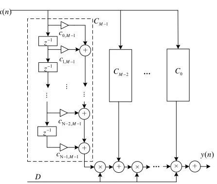
Figure 2. Block diagram of implementation of Farrow filter method.
The fractional time delay filter implemented by Farrow structure is one of the filters receiving the most attention in recent years with its implementation shown in Figure 2. Assuming the frequency response of the fractional time delay filter is written as:
1
0
( ) N ( ) j n n n
H C D e
(18)Where the filter coefficient of the above formula is expressed by multinomial:
1 , 0
( ) M m
n n m
m
C D C D
(19)Then, the following can be obtained:
1 1 , 0 0
( ) N M m j n
n m n m
H C D e
(20)The Farrow structure is designed to calculate the coefficient Cn m, to enable it to satisfy the following formula: 1 1 0 0 1 1 , 0 0 min
D N M
m j n j D
n m
n m
D
C D e e dDd
(21) Where
[ , ]0 1 denotes band width of fractional time delay at digital frequency,0 1
[ , ]
D D D denotes the range of parameters of fraction time delay. The number of order of the filter
Performance Analysis
To verify the influence of accurate time delay compensation method on signals, two paths of broad-band LFM signals are generated by MATLAB simulation for verification. The LFM signals are less relevant to various environmental noises and easy to detect. Its mathematical expression is as follows:
2 0
1
( ) cos{2 ( [ ( 1)] [ ( 1)] )} 2
i i
x n A f nD i K nD i (22)
Where Ai refers to the amplitude value of LFM, f0 and K refer to its initial frequency and FM
slow respectively and K B T/ whereB refers to signal bandwidth and T refers to time length of intercepting signals.
To determine whether or not the two signals that are processed by time delay are fully consistent in terms of time, we select correlation coefficient of the two signals for measuring them. The correlation coefficient can be expressed in the following formula:
1 1 1
2 2
1 1 1 1
1 1
( ) ( ) ( ) ( )
1 1
( ) ( ) ( ) ( )
N N N
i i j j
n m m
ij
N N N N
i i j j
n m n m
x n x m x n x m
N N
x n x m x n x m
N N
(23)
It may be seen from the above formula that if the two signals are fully consistent, 1; if there is time delay error between the two signals, 1 where the smaller the time delay error between the signals is, the larger the correlation coefficient is.
Different sampling rates and the same time delay
The true value of time delay between two signals is fixed as D5.45. The conventional time
delay method (Nearest Neighbor), linear interpolation method, rectangular windowed Sinc function interpolation method, Lagrange interpolation method and Farrow filter method are respectively utilized to perform time delay processing on the signals. Since f01kHz and B4kHz , the
sampling rate must be fS 10kHz, selecting fS[12 40], kHz. For different sampling rates, we use
different time delay methods for processing the signals. The correlation coefficient is obtained by solving two paths of signals to compare the correlation of the signals.
Figure 3. Comparison of performances of different time delay methods at different sampling rates.
The Same Sampling Rate and Different time Delays
The true value of the time delay between the two signals is fixed asD[5.0,5.5], selecting LFM
0 1
f kHz,B4kHzand the sampling rate of the signals is fS 12kHz.
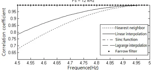
Figure 4. Comparison of performance of different time delay methods with different time delays.
We may find in Figure 4 that the correlation of the signals are the best with correlation coefficient up to 0.98 when rectangular windowed Sinc function interpolation method, Lagrange interpolation method and Farrow filter method are used for signal time delay compensation. The curves of their correlation coefficients in the Figures are overlapped. With increasing time delay error, the correlation of the signals is worsening after the conventional time delay method and linear interpolation method are used for signal time delay compensation.
Influence on Formation of Sonar Beam
[image:6.612.143.459.302.443.2]0 50 100 150 200 250 300 350 0
0.1 0.2 0.3 0.4 0.5 0.6 0.7 0.8 0.9 1
0 50 100 150 200 250 300 350
[image:7.612.113.499.73.421.2] [image:7.612.311.500.75.219.2]0 0.1 0.2 0.3 0.4 0.5 0.6 0.7 0.8 0.9 1
Figure 5. Results of conventional time delay. Figure 6. Results of accurate time delay.
Figure 7. Comparison of results of conventional time delay and accurate time delay. It can be seen from Figure 5-7 by comparison:
(1) The conventional time delay algorithm generates more false peaks with unsmooth beam formation diagram while accurate time delay algorithm has smoother beam formation diagram without false peaks.
(2) The accurate time delay algorithm is lower than conventional time delay algorithm in terms of side lobe.
(3) The accurate time delay algorithm has the same beam width with conventional time delay algorithm. This is because the beam width is mainly determined by array aperture and working frequency.
Conclusion
This paper analyzes the influence of time delay accuracy on sonar beam formation by studying theory and simulation of conventional time delay and accurate time delay algorithms. The simulation results show that
(1) Sinc function interpolation method, Lagrange interpolation method and Farrow filter method etc. have better performance of correlation.
[image:7.612.203.407.249.413.2]References
[1] X.F. Zhang, F. Wang, D.Z. Xu, et al. Theory and Application of Array Signal Processing. Beijing, National Defense Industrial Publishing House, 2010.
[2] Q.H. Li, Introduction to Sonar Signal Processing. Beijing, Navy Publishing House, 2000. [3] Q.H. Li, Designing Principle of Digital Sonar. Hefei, Anhui Education Press, 2003.
[4] T. Tian, G.Z. Liu, D.J. Sun, Sonar Technology. Harbin, Harbin Engineering University Press, 2006.
[5]Z.C. Fan, H.Y. Li, Z.S. He. Wideband digital array beam-forming based on fractional delay, 2008, 6(6): 450-453.
[6]C.L, Y.C. Bai, X.G. Zhang. Improved fractional time delay estimation method and its application, 2015, 30(6): 1279-1285.
[7]H.C. So. Adaptive TDOA estimation in presence of impulsive noise, Electronics Letters, 1998, 34(15): 1455-1456.
[8]Qin B., Zhang H., Fu Q., et al. Subsample time delay estimation via improved GCC PHAT algorithm [C]//2008 9th International Conference on Signal Processing. Signal Processing, IEEE, 2008: 2579-2582.
[9]Y. Guo, T.S. Qiu. A new time delay estimation method based on lagrange interpolation filter in implllsive noise environment, Journal of Electronics & Information Technology, 2007, 29(9): 2038-2041.
[10]S.R. Dooley, A.K. Nandi. Adaptive sub-sample time delay estimation using lagrange interpolators, IEEE Trams. On Signal Processing Letter, 1999, 6(3): 65-67.
[11]H. Sha, X.M. Huang, X. Zhang, et al. Method of pseudo-range Doppler simulation in navigation channel simulator on VFD filter, Journal of National University of Defense Technology, 2014, 36(4): 61-65.
[12]Y.J. Zhai, J.X. Hu, R.G. Li. Design of Fractional Time Delay Filter in Broadband Beam Forming, 2014, 37(10): 110-113.