University of Huddersfield Repository
Konstantinos, Michail, Zolotas, A.C. and Goodall, Roger M.
SimulationBased Optimum Sensor Selection Design for an Uncertain EMS System Via Monte
Carlo Technique
Original Citation
Konstantinos, Michail, Zolotas, A.C. and Goodall, Roger M. (2011) SimulationBased Optimum
Sensor Selection Design for an Uncertain EMS System Via MonteCarlo Technique. In: 18th IFAC
World Congress, 28th August 2nd September 2011, Milan, Italy.
This version is available at http://eprints.hud.ac.uk/id/eprint/17749/
The University Repository is a digital collection of the research output of the
University, available on Open Access. Copyright and Moral Rights for the items
on this site are retained by the individual author and/or other copyright owners.
Users may access full items free of charge; copies of full text items generally
can be reproduced, displayed or performed and given to third parties in any
format or medium for personal research or study, educational or notforprofit
purposes without prior permission or charge, provided:
•
The authors, title and full bibliographic details is credited in any copy;
•
A hyperlink and/or URL is included for the original metadata page; and
•
The content is not changed in any way.
For more information, including our policy and submission procedure, please
contact the Repository Team at: [email protected].
Simulation-based Optimum Sensor
Selection Design for an Uncertain EMS
System via Monte-Carlo Technique.
?
Konstantinos Michail∗
Argyrios C. Zolotas, Roger M. Goodall∗∗
∗
Energy, Environment and Water Research Center, The Cyprus Institute, Nicosia, Cyprus (e-mail: kon [email protected])
∗∗
Control Systems Group, Department of Electronic and Electrical Engineering, Loughborough University, Loughborough, UK (e-mail:
{a.c.zolotas, r.m.goodall}@lboro.ac.uk)
Abstract: Optimum sensor selection in control system design is often a non-trivial task
to do. This paper presents a systematic design framework for selecting the sensors in an optimum manner that simultaneously satisfies complex system performance requirements such as optimum performance and robustness to structured uncertainties. The framework combines modern control design methods, Monte Carlo techniques and genetic algorithms. Without losing generality its efficacy is tested on an electromagnetic suspension system via appropriate realistic simulations.
Keywords:optimum sensor selection, modern control design, EMS systems, Monte Carlo, genetic algorithms
1. INTRODUCTION
Selecting the output measurements for controlling a sys-tem in an optimum manner is not a trivial task to do espe-cially if many candidate sensor sets exist. The complexity, the often conflicting closed-loop objectives, the constraints and other control properties like optimum performance, robust performance and sensor fault tolerance make the problem even more complicated. Although the research community has considered the sensor selection before [Wal and Jager 2001] no systematic framework has been devel-oped as flexible as the one presented in this paper able to handle many different conflicting closed-loop performance objectives subject to optimum sensor set selection. The novel sensor framework that is presented by the authors actually simplifies the sensor selection while ensuring the desired closed-loop response, optimum performance and robustness to structure uncertainties. The proposed sen-sor framework is very flexible and has been tested using various control strategies with many extensions developed by Michail [2009]. In this work, the framework is extended towards optimum sensor selection with robust performance and stability for an uncertain system. The key point of the approach is by incorporatingMonteCarlo (MC) methods (see Roberto et al. [2004]) with the constraint handling techniques (that are used in Genetic Algorithms (GA)). This idea has been roughly discussed before by the authors [Michail et al. 2008] but here a comprehensive description of the method is done along with appropriate simulations.
? The Authors would like to thank Engineering and Physical Sci-ences Research Council, UK, for supporting this research work under the project Grand Ref. EP/D063965/1, and in part under the NEW-ACE project ref. EP/E055877/1, and BAE Systems from Systems Engineering Innovation Centre, UK.
The proposed systematic framework combines the H∞
LoopShapingDesignProcedure (LSDP) [McFarlane and Glover 1992], the GAs [Konak et al. 2006] and MC method for robustness assessment.
TheElectro-MagneticSuspension (EMS) systems are be-ing used on theMAGnetic LEVitated trains [Lee et al. 2006]. As indicated by Goodall [2008] the EMS system is a non-linear, inherently unstable system with non-trial requirements and it can easily serve as a good example for testing the efficacy of the proposed framework.
This paper is separated into five sections: Section 2 de-scribes the EMS model and the closed-loop requirements of the EMS. In Section 3 the details of the framework are given. Section 4 discusses the simulation results and the efficacy of the proposed framework is assessed. The paper concludes by summarizing the advantages in Section 5.
2. EMS MODELLING AND REQUIREMENTS
2.1 The EMS Model
The single degree-of-freedom model represents the quarter of a typical MAGLEV vehicle and is analysed here. As shown by Goodall [2004] a single-stage electro-magnetic suspension is suitable for low speed vehicles. The basic quarter car diagram of the MAGLEV vehicle is shown in Fig. 1. The suspension consists of an electromagnet with a ferromagnetic core and a coil ofNcturns which is attracted
to the rail that is made of ferromagnetic material. The carriage mass (Ms) is attached on the electromagnet, with
zt the rail’s position and z the electromagnet’s position.
The airgap (zt −z) is to be controlled so as to vary
zt z
[image:3.595.312.557.69.223.2] [image:3.595.83.256.75.198.2] [image:3.595.102.286.341.434.2] [image:3.595.333.527.468.533.2]Msg
Fig. 1. Single-stage suspension for MAGLEV vehicles.
flux densityB, airgapGand the coil’s currentI that give non-linear characteristics to the suspension as described in Goodall [2008]. Assuming that the motion vertically downwards is taken as positive the non-linear model of the EMS system is described by Newton’s equation of motion in (1) and the voltageVcin (2) across the electromagnet’s
coil from Kirchoff’s law. Equations (3) and (4) give the force and flux density and the airgap velocity respectively [Goodall 2008].
Ms
d2Z
dt2 =Msg−F (1) Vc =IRc+LcdI
dt +NcAp dB
dt (2) B=KbI
G, F=KfB
2 (3) dG dt = dzt dt − dZ dt (4)
where g is the gravity acceleration constant which is 9.81m/s2. The linearisation of the non-linear MAGLEV suspension model is based on small perturbations around the operating point. The following definitions are used with lower case letters defining the small variation around the operating point and subscript ’o’ referring to the operating point.
B=Bo+b, F =Fo+f (5)
I=Io+i, G=Go+ (zt−z) (6)
Vc=Vo+uc, Z=Zo+z (7)
Following the linearization procedure as given by Goodall [2008] the state space description of the EMS system can be expressed in state space form as in (8) where the selected states are x = [i z˙ (zt−z)]T and the output
equation corresponds to the following five measurements: ithe coil’s current, bthe flux density, (zt−z) the airgap,
˙
zthe vertical velocity and ¨z the vertical acceleration. The matricesA, Buc, Bz˙t andC are given by (9)-(11).
˙
x=Ax+Bucuc+Bz˙tz˙t (8)
y=Cx
A=
− Rc
Lc+KbGNcoAp
− KbNcApIo
G2
o
Lc+KbGNcoAp
0
−2Kf
Io
MsG2o
0 2Kf
I2
o
MsG3o
0 −1 0
(9)
Buc =
1 Lc+KbNGocAp
0 0
, Bz˙t =
KbNcApIo
G2
o
Lc+KbNGocAp 0 1 (10) C=
1 0 0
Kb
Go
0 −KbIo
G2
o
0 0 1
0 1 0
−2Kf Io
MsG2o
0 2Kf I
2
o
MsG3o (11)
The output matric, C gives the five measurements (i.e. i,b,(zt−z), ˙z and ¨z) and the sensor sets can be obtained
by using the corresponding rows of C in (11). The total number of sensor sets is Ns = 2ns −1, where ns is the
total number of sensors. Given that the EMS system has 5 outputs there are 31 candidate sensor sets. However, since the LSDP controller design technique is used here and therefore the airgap measurement is a standard mea-surement, the number of candidate sensor sets reduces to 15. The electromagnet design of MAGLEV vehicles is described in more details by Goodall [Sep 1985]. A typical quarter car vehicle of 1000kg requires an operating force of Fo = Ms×g. The operating airgap (Go) is at 15mm
to accommodate the track roughness. According to these requirements the rest of the parameters can be calculated and they are listed on Table 1.
[image:3.595.39.294.650.755.2]The EMS system is inherently unstable system and is also characterised by uncertainties that can be caused from various reasons. Table 1 tabulates the uncertainties that could possibly occur.
Table 1. Parameters of the EMS system.
Par. Val. Unc. Par. Val. Unc.
Go 0.015m 10% Ms 1000kg 10%
Bo 1T 10% Rc 10Ω 50%
Io 10A 10% Lc 0.1H 50%
Vo 100V 0% Nc 2000 0%
Fo 9810N 10% Ap 0.01m2 0%
Note: Par. - Parameter, Val. - Value, Unc. - Uncertainty
2.2 Design Requirements and Inputs to the EMS
Stochastic Inputs The stochastic inputs are random vari-ations of the rail position as the vehicle moves along the track. This is caused by the steel rail installation discrep-ancies due to track-laying inaccuracies and unevenness. Considering the vertical direction, the velocity variations can be approximated by a double-sided power spectrum density (PSD) expressed as
Sz˙t =πArVv (12)
whereVvis the vehicle speed (taken as 15m/sin this case)
andArrepresents the roughness which is assigned a value
as 1×10⁻⁷
m corresponding to high quality track. Then the corresponding autocorrelation function is given as:
R(τ) = 2π2ArVvδ(τ) (13)
quantities (acceleration, current etc) using time history data.
Deterministic Input The main deterministic input to the suspension in the vertical direction is due to the transition onto a gradient. In this work, the deterministic input (see Fig. 2) is a gradient of 5% at a vehicle speed of 15m/s, an acceleration of 0.5m/s2 and a jerk of 1m/s3.
! " # $ % & ' (
!
!)&
"
")&
#
#)&
$
$)&
%
%)&
*+, - ./0 12
2
3
4
3
5
6
789
:
;< => ?@A
B
3
49
2
8
7C ;<
=
>
@A
D
9
>
789
:
;<
@
←EFF
-G-HIJ+KL
←M
K/+J+KL
↑N-GK
F
[image:4.595.62.274.167.325.2]+JO
Fig. 2. Deterministic input to the suspension with a vehicle speed of 15ms−1
and 5% gradient.
EMS Control Properties The design requirements for an EMS system depend on the type and speed of the train. and they are well described in Goodall [1994, 2004]. His work is focused upon the low speed Birmingham Airport Maglev vehicle EMS suspension requirements which op-erated successfully in the UK for a period of 12 years in the 1980s and 1990s. Fundamentally, there is a trade-off between the deterministic and stochastic responses of the EMS system. Table 2 tabulates the design limitations for the deterministic and stochastic features. The deter-ministic features are limited to the maximum standard values and the stochastic ones are set as objectives to be minimized i.e. the vertical acceleration ¨zrms(improve ride
quality) and the RMS current variations irms from the
stochastic response.
The robust stability margin (degree of robustness) calcu-lated from the LSDP is maximized for maximum robust-ness to uncertainties (note thatγ= 1/).
Since noise affects the sensors, an amount of this noise will appear on the control effortunrms [Michail et al. 2009]. In
that case the noise, if not eliminated, can be amplified from the controller hence its been set as an objective to be minimised.
Summarizing, the objective functionsφi to be minimized
are formally written as:
φ1=irms, φ2=γ, φ3= ¨zrms, φ4=unrms (14)
3. THE SENSOR OPTIMISATION FRAMEWORK
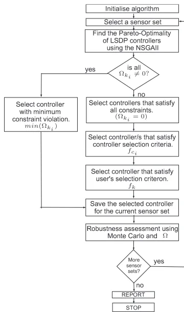
The proposed framework can be summarised in the flow chart of Fig. 3. The particular points include the use of
H∞ loop-shaping design and the heuristic optimisation
(evolutionary algorithms) method for tuning the controller subject to strict requirements (objectives and constraints)
Table 2. Constraints on the EMS system per-formance.
EMS limitations Value
RMS acceleration,¨zrms ≤1ms−2
RMS airgap variation,(zt−z)rms ≤5mm
RMS control effort,ucrms ≤300V(3I0Rc)
Maximum airgap deviation,(zt−z)p ≤7.5mm
Control effort,ucp ≤300V(3I0Rc)
Settling time,ts ≤3s
Airgap Steady state error,(zt−z)ess = 0
Robust Stability Margin, ≥0.15
for each feasible sensor set of the EMS system.
Prior to running the algorithm (initialization phase), some parameters are assigned including evolutionary algorithms parameters, controller selection criteria (fci) and the user’s
controller selection criterion (fk). fci and fk make sure
that the selected controller results in a desired closed-loop performance. Starting the optimisation procedure, the first sensor set is selected and the evolutionary algorithm seeks the Pareto-optimality of the objective functions in (14) (i.e. the trade-off between them) subject to the constraints listed on Table 2.
In the sequence, the algorithm seeks to find the
opti-PQ RSRT URVW T UX Y ZRS[\ ] W UW^ST VW QVY ZVW S
_ `ab
c
bd
c
`a
c
be cf
g
W V
hij k ] W UW ^S^Y QSZY UUW ZV S[TS VTSRVl
g
T UU^Y QVSZT RQSV m
] W UW ^S^Y QSZY UUW ZS[T SVTSRVl
g
n
VW ZoV VW UW^SRY Q ^ ZRSW ZY Qm
QY p RQq S[W r T ZW SYst uSR\ T URS
g
Y l v] w r ^Y QSZY UUW ZV
n
V RQX S[W x ] y z PP
{ | kj { i
]
W UW ^S^Y QSZY UUW Z
}
RS[ \ RQ R\
n
\
^Y QVSZT RQS~ RY UTSRY Qm
g
W V
QY RV T UU
] T~W S[W VW UW ^SWq ^Y QSZY UUW Z lY ZS[W ^
n
ZZW QSVW QVY ZVWS
]
W UW ^S^Y QSZY UUW ZV S[TS VT SRVl
g
^Y QSZY UUW ZVW UW^SRY Q ^ ZRSW ZRT m
Y
n
VSQWVV TVVW VV \ W QS
n
V RQX Y QSW T ZUY T Qq
(Ωki= 0)
min(Ωki)
Ωki6= 0?
Ω
fci
[image:4.595.339.519.336.640.2]fk
Fig. 3. Flow chart of the proposed sensor optimisation framework with robustH∞ loop-shaping design.
mized controller by using the overall constraint violation function,Ω (see (17) in Section 3.2). At this point there are two paths to follow:
(i) If there is no sufficient controller (this can be easily verified by checking Ω for each individual response) then the controller which gives the minimum Ω is selected and saved.
step is to select those controllers that satisfy the controller selection criteria fci and finally, the user’s controller
se-lection criteria, fk is used to select the controller which
results in the desired closed-loop response. If no controller exists to satisfy fci then the algorithm directly selects a
controller based only onfk. The optimally tuned controller
is saved and the algorithm moves to the next stage where robustness is assessed via MC method.
The particular sensor set and the selected controller pro-vide a nominal performance that is assessed for parametric uncertainties by combining the MC method with the over-all constraint violation function in the following way: (i) For every qth of the uncertain EMS system do: cal-culate the overall constraint violation function (Ω) using simulation results from the closed-loop response of the deterministic and stochastic profiles of the track.
(ii) From the closed-loop responses of theQsamples select the one with the maximum value of the overall constraint violation function. This is taken as the worse case overall constraint violation function noted as (Ωw−c). In case the
closed-loop response with an uncertain model is unstable, Ωw−c is quantified by infinity.
In this way the robustness of the optimally tuned nominal controller is assessed. Finally, the algorithm moves to the next feasible sensor set until all feasible sensor sets are checked as described above.
3.1 H∞ loop-shaping design
The design of the optimised controller is based on the nor-malised coprime-factor plant description, proposed by Mc-Farlane and Glover [1992], which incorporates the simple performance/robustness tradeoff obtained in loop shaping, with the normalised left coprime factorization robust sta-bilization method as a means of guaranteeing closed-loop stability.
The design method proceeds by shaping the open-loop characteristics of the plant by means of the weighting functions W1 and W2 (see Fig. 4(a)). The plant is tem-porarily redefined as ˆG(s) =W2GW1 and the H∞
opti-mal controller ˆK(s) is calculated. In the final stage, the weighting functions are merged with the controller by defining the overall controller K(s)=W1 ˆKW2 as shown in Fig. 4(b). The size of model uncertainty is quantified
u y
G(s) ˆ
K(s)
(a)Shaped plant.
u y
ˆ K(s)
K(s)
[image:5.595.48.284.566.642.2](b)Final controller.
Fig. 4.H∞loop-shaping design.
by the stability radius (refer to McFarlane and Glover [1992] and Skogestad and Postlethwaite [2005] for more details), i.e. the stability margin. For values of ≥ 0.25, 25% coprime factor uncertainty is allowable. However, in this paper the coprime factor uncertainty is set to 15% i.e. ≥0.15.
In typical design the filter functions and thus the controller are to be kept as simple as possible. Thus, the W1 pre-compensator, is chosen as a single scalar weighting
func-tion set to unity. For theW2 post-compensators there can be five weighting functions that are used depending on the selected sensor set. The airgap (zt−z) measurement
is a compulsory measurement required for proper maglev control of the magnet distance from the rail and thus a low pass filter (W(zt−z)) is chosen with integral action
allowing zero steady state airgap error (for the nominal performance). The weighting functions are given as
W1 = 1; W2 =diag(Wi, Wb, W(zt−z), W˙z, W¨z) (15)
with,
W(zt−z)=
s Mp1/np
+ωb
s+ωbA1p/np
np
(16)
The above results in a minimum phase and stable weight-ing filter with roll-off rate np. Note that there exist 24
candidate sensor sets and that the airgap sensor is always required.
3.2 Multi-objective Constrained Optimisation
Heuristic approaches are very powerful optimisation tools which are used in many engineering problems. Particularly the GAs have been extensively implemented in control engineering (see Fleming and Purshouse [2002]). Differ-ent types of GAs have been developed in recDiffer-ent years and they are well summarized by Konak et al. [2006]. In this research work, the recently developed GA based on non-dominated sorting of the population,Non-dominated
Sorting Genetic Algorithm II (NSGA-II) is used that proves to be a powerful optimization tool. For the inter-ested reader details on NSGA-II are described by Deb et al. [2002]. NSGA-II is an evolutionary process that requires some parameters to be assigned in order to ensure proper population convergence towards Pareto-optimality. These are mainly selected from experience rather than from a-priori knowledge of the optimisation problem. The crossover probability is generally selected to be large in order to have a good mix of genetic material. The crossover probability is set to 90% and the mutation probability is defined as 1/nuwhere,nu is the number of variables. The
population consists of 50 chromosomes and the stopping criterion is the maximum generation numberNgen. Ngen
has a significant role on the Pareto-Optimality and the computational time i.e. the higher the generation number is the longer the computational time but it is more possible for the evolved population to converge and finally spread onto the optimum Pareto front.Ngendepends among other
factors on the number of variables to be tuned because the larger the number of variables is a largerNgenis required
with the expense of having longer computational time. In this problem because the number of variables varies according to the number of sensors,Ngen is set at 200 for
sensor sets with up to 3 sensors and for the rest including the full sensor set is set at 250 generations.
Michail [2009]. This method is using a function in order to ’guide‘ the objective functions in (14) towards the Pareto-optimality while the desired constraints on Table 2 are satisfied. The overall constraint violation function is given as
Ω(k(j), f(i)) =
J X
j=1
ωj(k(j)) + I X
i=1
ψi(f(i)) (17)
where,ωjis the jthsoft constraint violation for the
corre-spondingjth quantity to be constrained (k) and J is the total number of soft constraints. Similarly, ψ is the hard constraint violation for theith quantity to be constrained
(f). The overall constraint violation function serves as a controller selection criterion within the systematic frame-work as described at the beginning of this section.
3.3 Robustness assessment within the framework
Taking advantage of the fact that any changes in the closed-loop response (both stability and performance) will be reflected on Ω in (17), robustness against paramet-ric uncertainties can be tested in combination with MC technique. MC technique has been used in a variety of disciplines for many years now therefore the details are omitted. Monte Carlo is a probabilistic method that can be used to randomly sample the uncertain parameters of the EMS system and them to test the closed-loop stability and performance. This can be achieved by using a number of samples,Qof the uncertain EMS and test them using the nominal controller. In this paper 100 samples (Q= 100) of the EMS model are tested for each sensor set. Then, the case value of Ω is taken that represents the worse-case response noted as Ωw−c.
4. SIMULATIONS AND DATA ANALYSIS
The framework is tested in MATLAB R2009b simulation environment without Java function due to large computa-tional need (simulation based). The computer used is the powerful DELL T610 with 2.93GHz IntelrXeonrX5570 processor and 8GB RAM.The average simulation time per sensor set is about 2.5 hours while completion of the framework takes around 45 hours.
The controller selection criteria (fci, fk) for the desired
closed-loop response are given as follows
fc1 ≡z¨rms≤0.5m/s2, fc2 ≡unrms ≤10V, (18)
fk≡max() (19)
Recall that if fci criteria are not satisfied then the best
controller selection is done based only on fk. The first
set of closed-loop desired characteristics in (18) ensures that the controllers to be selected are within the limits indicated while the last criterion in (19) ensures that the selected controller has the maximum robust stability margin (maximum robustness).
From the results it was found that the proposed systematic framework is able to identify stabilizing controllers that satisfy (17),(18) and (19) for 11 out of 16 sensor sets. The other four violate (17) hence the performance is not satisfactory. However, they could be used if the constraint violation does not threaten the safety of the system. Table 3 lists some sensor sets that are selected for compre-hensive analysis of the results. The second column lists the
sensor sets and the first the corresponding identification number. The next four columns are the variables from the closed-loop response with the stochastic track profile and the further four show the variable values from the deter-ministic profile. The next column is the resulting stability margin from the H∞ loop-shaping design and the 12
th
column lists the resulting RMS level of the noise on the input voltage. The 13th column shows whether the overall
constraint violation function, Ω is satisfied or not (without any uncertainties i.e. the nominal closed-loop response). The last column represents the worse-case overall violation function, Ωw−c. That is the maximum value of Ω among
the resulted closed-loop responses using theQsamples of the uncertain EMS system. If the worst-case response is instability of the closed-loop then the Ωwc is assigned to
be infinity.
Inspecting the Ω column that reflects the nominal perfor-mance of the EMS system it can be seen that id:1 and 2 violate the stability margin while the rest of the sensor sets satisfy it. Comparing the EMS performance with id:8 (i.e. the full sensor set) and the rest of the sensor sets is ob-served that similar nominal response can be achieved with fewer sensors eg. id:3. However, when the performance against parametric variations is assessed with Monte Carlo it becomes difficult to achieve robustness while in some cases the worst case is instability eg. id:1. The sensor set id:1 has a value of infinity Ωw−c which means that there
is a combination of uncertain EMS parameters that cause instability. The best robust performance is achieved with id:7 comprising of 4 sensors and it gives a Ωw−c of 1.21
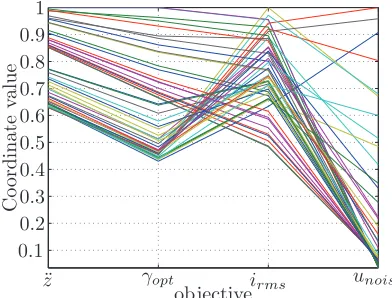
that means for a particular combination of the uncertain parameters there is some control constraint violation. Nev-ertheless, this is the best sensor set with which robust performance of the EMS system can be achieved. Figure 5 depicts the Pareto-Optimality with id:7 (note that the values are normilized around one for good resolution). It is clear that the trade-off between the objective func-tions is successfully found. Figure 6 illustrates the airgap deflections of the closed-loop response with the nominal controller and the deterministic input (the transition onto the track’s gradient) by sampling 100 uncertain non-linear models of the suspension. The response of the suspension is restricted to the requirements as listed in Table 2. Al-though the steady state error is not zero is still very small and does not impose any serious danger for the operation of the suspension.
objective
C
o
or
d
in
at
e
va
lu
e
¨
z γopt irms unoise
[image:6.595.331.527.589.738.2]0.1 0.2 0.3 0.4 0.5 0.6 0.7 0.8 0.9 1
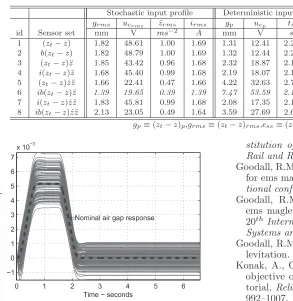
Table 3. Optimised sensor configurations for the EMS system.
Stochastic input profile Deterministic input profile
grms ucrms ¨zrms irms gp ucp ts ess unrms Ω Ωw−c
id Sensor set mm V ms−2 A mm V s V
1 (zt−z) 1.82 48.61 1.00 1.69 1.31 12.41 2.29 X 0.14 0.26 x ∞
2 b(zt−z) 1.82 48.79 1.00 1.69 1.32 12.44 2.29 X 0.14 0.26 x 145
3 (zt−z)¨z 1.85 43.42 0.96 1.68 2.32 18.87 2.19 X 0.15 0.17 X 23.34
4 i(zt−z)¨z 1.68 45.40 0.99 1.68 2.19 18.07 2.18 X 0.15 0.17 X 38.80
5 (zt−z) ˙zz¨ 1.66 22.41 0.47 1.66 4.22 32.63 2.73 X 0.15 0.47 X 27.77
6 ib(zt−z)¨z 1.39 19.65 0.39 1.39 7.47 53.59 2.16 X 0.15 0.45 X 1.21
7 i(zt−z) ˙z¨z 1.83 45.81 0.99 1.68 2.08 17.35 2.19 X 0.15 0.17 X 67044
8 ib(zt−z) ˙zz¨ 2.13 23.05 0.49 1.64 3.59 27.69 2.68 X 0.15 0.45 X 24.59
gp≡(zt−z)p,grms≡(zt−z)rms,ess≡(zt−z)ess
¡
¢
£¤ ¥¦¤
§
¨
© ª« ¬® ¯
°
¯
±
⇐² ³ ´³ µ ¶ ³ · µ
·
[image:7.595.70.363.84.385.2]
Fig. 6. Airgap deflections with 100 samples of the uncertain EMS using the sensor set with id:6.
5. CONCLUSION
This paper has shown that the proposed framework is able to identify the best sensor set with which the control of EMS system is possible subject to multiple and complex requirements that otherwise would be very difficult to achieve by manual design of the control system. It has been showed that with id:7 it is possible to control a complex electromechanical system like the EMS with non-linearities, uncertainties and multiple constrained control objectives. The framework is very flexible and without losing generality it can be easily adapted to many sensor selection problems in control systems provided that the dynamic model is well known.
REFERENCES
Coello, C.A.C. (2002). Theoretical and numerical constraint-handling techniques used with evolutionary algorithms: A survey of the state of the art. Computer Methods in Applied Mechanics and Engineering, 191(11-12), 1245–1287.
Deb, K., Pratap, A., Agarwal, S., and Meyarivan, T. (2002). A fast and elitist multiobjective genetic al-gorithm: Nsga-ii. IEEE Transactions on Evolutionary Computation, 6(2), 182–197.
Fleming, P.J. and Purshouse, R.C. (2002). Evolutionary algorithms in control systems engineering: A survey.
Control Engineering Practice, 10(11), 1223–1241. Goodall, R.M. (1994). Dynamic characteristics in the
design of maglev suspensions. Proceedings of the
In-stitution of Mechanical Engineers, Part F: Journal of Rail and Rapid Transit, 208(1), 33–41.
Goodall, R.M. (2004). Dynamics and control requirements for ems maglev suspensions. InProceedings on interna-tional conference on Maglev, 926–934.
Goodall, R.M. (2008). Generalised design models for ems maglev. In Proceedings of MAGLEV 2008 - The
20thInternational Conference on Magnetically Levitated
Systems and Linear Drives.
Goodall, R.M. (Sep 1985). The theory of electromagnetic levitation. Physics in Technology, 16(5), 207–213. Konak, A., Coit, D.W., and Smith, A.E. (2006).
Multi-objective optimization using genetic algorithms: A tu-torial.Reliability Engineering and System Safety, 91(9), 992–1007.
Lee, H.W., Kim, K.C., and Lee, J. (2006). Review of maglev train technologies. IEEE Transactions on Magnetics, 42(7), 1917–1925.
McFarlane, D.C. and Glover, K. (1992). A loop-shaping design procedure using h∞ synthesis. IEEE
Transac-tions on Automatic Control, 37(6), 759–769.
Michail, K. (2009). Optimised configuration of sensing elements for control and fault tolerance applied to an electro-magnetic suspension system. PhD dissertation, Loughborough University, Department of Electronic and Electrical Engineering. http://hdl.handle.net/2134/5806.
Michail, K., Zolotas, A.C., and Goodall, R.M. (2009). Ems systems: Optimised sensor configurations for control and sensor fault tolerance. Japan Society of Mechan-ical Engineers, International Symposium on Speed-up, Safety and Service Technology for Railway and Maglev Systems.
Michail, K., Zolotas, A.C., Goodall, R.M., and Pearson, J.T. (2008). Maglev suspensions - a sensor optimisa-tion framework. In 16th Mediterranean Conference on
Control and Automation, 1514–1519.
Roberto, T., Giuseppe, C., and Fabrizio, D. (2004). Ran-domized Algorithms for Analysis and Control of Uncer-tain Systems. Springer.
Skogestad, S. and Postlethwaite, I. (2005). Multivariable Feedback Control Analysis and Design. John Wiley & Sons Ltd, 2ndEdition, New York.

![Fig. 4.[1992] and Skogestad and Postlethwaite [2005] for moreby the stability radiusdetails), i.e](https://thumb-us.123doks.com/thumbv2/123dok_us/356622.1036806/5.595.48.284.566.642/fig-skogestad-postlethwaite-moreby-stability-radiusdetails-i-e.webp)