SRC RR 131A pdf

December, 1994

SRC

131a

The Juno-2 Constraint-Based

Drawing Editor

Allan Heydon and Greg Nelson

d i g i t a l

Systems Research Center

130 Lytton Avenue

Systems Research Center

The charter of SRC is to advance both the state of knowledge and the state of the art in computer systems. From our establishment in 1984, we have performed basic and applied research to support Digital’s business objectives. Our current work includes exploring distributed personal computing on multiple platforms, network-ing, programming technology, system modelling and management techniques, and selected applications.

Our strategy is to test the technical and practical value of our ideas by building hardware and software prototypes and using them as daily tools. Interesting systems are too complex to be evaluated solely in the abstract; extended use allows us to investigate their properties in depth. This experience is useful in the short term in refining our designs, and invaluable in the long term in advancing our knowledge. Most of the major advances in information systems have come through this strategy, including personal computing, distributed systems, and the Internet.

We also perform complementary work of a more mathematical flavor. Some of it is in established fields of theoretical computer science, such as the analysis of algorithms, computational geometry, and logics of programming. Other work explores new ground motivated by problems that arise in our systems research. We have a strong commitment to communicating our results; exposing and testing our ideas in the research and development communities leads to improved un-derstanding. Our research report series supplements publication in professional journals and conferences. We seek users for our prototype systems among those with whom we have common interests, and we encourage collaboration with uni-versity researchers.

The Juno-2 Constraint-Based

Drawing Editor

c

Digital Equipment Corporation 1994

Authors’ Abstract

Constraints are an important enabling technology for interactive graphics applica-tions. However, today’s constraint-based systems are plagued by several limita-tions, and constraints have yet to live up to their potential.

Juno-2 is a constraint-based double-view drawing editor that addresses some of these limitations. Constraints in Juno-2 are declarative, and they can include non-linear functions and ordered pairs. Moreover, the Juno-2 solver is not limited to acyclic constraint systems. Juno-2 also includes a powerful extension language that allows users to define new constraints. The system demonstrates that fast constraint solving is possible with a highly extensible, fully declarative constraint language.

The report describes what it is like to use Juno-2, outlines the methods that Juno-2 uses to solve constraints, and discusses its performance.

Perspective

Computers now handle the words in the documents that we write, and that is good: Revising, indexing, and formatting are lots easier, while hyperlinks have opened up shining vistas. Computers also handle the illustrations in our documents, but the news on that front is not so good. Producing accurate drawings is still a tedious task in many cases, revising them later is worse, and animations are not taking off as fast as hypertext. Even if we grant that a picture is worth a thousand words to the reader, why is its cost to the writer more like ten thousand?

If computers are ever to help illustrators as effectively as they help authors, some new ideas will be required. Juno-2 is a drawing editor that explores an intriguing collection of ideas about two-view editing, constraint-solving, and ex-tension languages. This brief report gives some early indications of the strengths and weaknesses of those ideas.

U N O

J

2

Constraint solver (2429) Virtual machine (2857) Compiler (9727) User interface (10140)

Predefined Juno-2 modules (5778)

Juno-2’s extensibility reaches three dimensions. Although you can’t tell it from the picture, Juno-2 modeled this tetrahedron in three-space. The edges were constrained to be equal, and the solver computed the coordinates of the vertices in three-space. You can move the tetrahedron in three-space by dragging the two-dimensional projections of its vertices.

A theorem of

projective geometry. A complete quadrilateral (the four black lines in the low-er half of the figure) has three pairs of opposite vertices. Draw lines from these six vertices through a point on a conic section. Each line intersects the conic section a second time. The three chords determined by the three pairs of second intersections are concurrent.

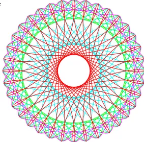
The predefined pie chart module is used here to show the number of lines of code in Juno-2

broken down by function. Juno-2 emulates Spirograph.

1

Introduction

This report describes Juno-2, an experimental, constraint-based, double-view drawing editor.

Constraints allow you to specify locations in your drawing declara-tively. For example, to draw an equilateral triangle, you first draw an arbitrary triangle and then constrain its sides to be equal; Juno-2 will adjust the vertices to make the triangle equilateral. Moreover, the constraints are maintained whenever part of the picture is changed, so constraints make it easier to maintain a picture in the face of modifications.

One of the novel things about Juno-2 is that it allows constraints to be defined in a powerful declarative extension language. This language makes it easy to define two-dimensional geometric constraints, which occur frequently in interactive graphics; but it is not limited to two dimensions or to geometry.

The Juno-2 extension language is imperative as well as declarative: it allows you to define new drawing operations as well as new constraints. You can write programs in Juno-2 the way some people write programs in PostScript, and execute them to produce pictures. But it is much more convenient to use Juno-2’s double-view editor, which displays a view of the picture as it would appear if printed and simultaneously displays a program in the Juno-2 language that draws the picture. You can edit in either view, and both views are updated.

We will describe what it is like to use Juno-2 and sketch the main techniques used to implement it, leaving the more technical details for later papers. We hope the report will appeal to anybody interested in graphical user interfaces, not only to specialists in constraint systems.

Contents

Introduction Simple drawings Templates and folding Juno-2 extensibility Drawing an S Modules

The constraint solver Performance Conclusions

Figure 2. As a test of extensibility, we im-plemented a Juno-2 module to draw bulleted slides with items and sub-items. This figure uses the module to show the table of contents of this report.

Interactive constraint-based graphics goes back to Ivan Sutherland’s pioneering program Sketchpad [19]. But there are many difficulties with constraints, and thirty years after Sketchpad, the sad fact is that constraints have so far been more promising than useful. The goal of our research is to identify and solve the problems that continue to prevent constraints from realizing their potential in interactive graphics. For example:

It is difficult to build a constraint solver that is fast and reliable.

Juno-2 uses a combination of symbolic and numeric techniques that seems quite promising.

Constraints are slippery. When a solver finds a solution to an

under-constrained system, it is often far from the solution the user intended. Juno-2 addresses this problem using hints: the solution for an un-known is chosen to be near the user-provided hint for that unun-known.

It can be difficult to design an interface that allows users to determine

constraints are visible in the program view, and can be modified or deleted in that view with ordinary text-editing operations.

The effective definition of constraints can require more mathematical

sophistication than most users have. We hope Juno-2’s program-mability will help with this problem, by allowing a collection of useful constraints and drawing operations to be defined once by an experienced Juno-2 user and then used many times by novices. Many other systems have similar goals. ThingLab [2] and Garnet [12] provide extensible constraint solvers. In these systems, users define constraints imperatively by providing functions to solve individual con-straints, and the solver attempts to invoke them in an order that solves them all. However, many useful constraint systems contain cycles and therefore cannot be solved by this method. In contrast, Juno-2 allows the user to define constraints declaratively. This can (and usually does) produce cyclic constraint systems; Juno-2 solves them with numerical methods.

Donald Knuth’s METAFONT [9] and John Hobby’s MetaPost [8] also provide numerical solvers, but these systems are limited to constraints that are algebraically linear. Unfortunately, this precludes important geometric predicates like parallelism and congruence. Chris Van Wyk’s IDEAL [20] solves a larger class of constraints, but not general non-linear constraints. These systems are programmable, but not WYSIWYG (what you see is what you get).

Constraint-based drawing programs like Michael Gleicher’s Briar [7], Steve Sistare’s Converge [18], and Aldus’s commercial program Intel-liDraw provide numerical non-linear constraint solving, but only over a fixed set of constraints. These systems are WYSIWYG, but provide no programming view.

2

2

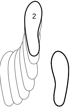
Figure 3. Count two of the man’s part of the basic step of the cha-cha. The figure was drawn by overlaying several frames of the animation. At each weight change, the count is displayed on the weighted foot.

Juno-1 [14], the predecessor of Juno-2, uses double-view editing to combine the WYSIWYG and programming paradigms. Juno-1 also pro-vides numerical non-linear constraint solving, but again for a fixed set of constraints. Although you can define new procedures with Juno-1, you cannot define new constraints. Since all constraints are specified in terms of four geometric primitives, using Juno-1 can be a bit like doing construc-tions with straightedge and compass.

Juno-2’s most important innovation is to allow an extensible class of nonlinear constraints. A Juno-2 user can introduce new constraints by declarative first-order predicate definitions, including definitions using ex-istential quantifiers. In addition, Juno-2 enriches the value space with ordered pairs, thereby making the constraint language much more expres-sive.

Juno-2 is still under development, but it is already a useful system. The figures in this report were all drawn using Juno-2 (except Figure 5, which is a screen snapshot). The application produces PostScript. As an experimental system, Juno-2 offers less ease of use than commercial drawing programs. But this must be weighed against the fact that most easy-to-use illustrators produce noticeably imperfect drawings, with arrowheads

that don’t point quite where they should, labels that aren’t centered, nodes that aren’t equally spaced, and so forth. These drawings are also tedious to modify. If you need to produce a precise drawing, Juno-2 has many advantages over the alternatives, such as programming directly in Postscript or using a CAD system.

The extensibility of the system makes it useful for experimenting with constraints in many different user interfaces. For example, we have used it to prototype user interfaces for drawing bulleted outlines for slides, for drawing scatter-plots and performance graphs, for drawing labeled directed graphs, and for editing constrained three-dimensional shapes by dragging their two-dimensional projections. Figures 1 and 2 contain images from some of these experiments.

We have also used Juno-2 to experiment with the interactive production of animations. An animation can be regarded as an underconstrained drawing in which one of the degrees of freedom represents time. We wish we could publish this report in a DynaBook with animated figures, but that isn’t yet possible. In the meantime, we have done our best to illustrate the flavor of the animations in Figures 3 and 4.

2

Simple drawings

Figure 5 shows a snapshot of the Juno-2 application after we have used it to draw an equilateral triangle. The triangle is displayed in the graphical

view, and its corresponding program is displayed in the textual program view.

In this section we will describe how the equilateral triangle was drawn, using it as an example of a typical simple drawing. In passing, we will describe some of the aspects of Juno-2 that are important in the rest of the report.

The standard recipe for making a simple drawing with Juno-2 has three steps: sketching, constraining, and adjusting. First you create a rough sketch of the drawing, then you tidy up the drawing by adding constraints, and finally you use the drag tool to fine-tune the drawing within the degrees of freedom that remain.

The user interface provides predefined tools for operating on the draw-ing. To apply a tool to some points in the drawing, you select the tool and click near the points. Both the drawing and program views are then modified to show the effect of the operation. Juno-2 has tools for creating, freezing (that is, fixing), and dragging points; for adding constraints

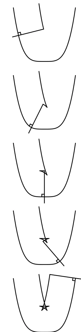
(ei-Figure 4. If you walk along the graph of the function y = x

4

carrying a beam that extends one unit to each side, the inner tip of the beam traces out a surprising five-pointed star, as discovered by Rida T. Farouki. The figure shows several frames from a Juno-2 animation of this phenomenon.

ther predefined or user-defined); and for adding drawing operations (either predefined or user-defined).

Sketching. To produce the triangle, we used the Create tool in the palette on the left to create three points, which the system automatically named a, b, and c. We then drew a filled triangle using the tools for

Figure 5. A screen snapshot of the Juno-2 user interface. Visible are: the palette of built-in tools; the palette for the predefined

PSmodule; the menu of predefined modules; the graphical view; and the program view.

module. The system simultaneously added variable declarations and draw-ing commands to the program view.

Here is a synopsis of thePSmodule, which provides the PostScript-like drawing operations used by Juno-2:

PS.MoveTo(p)starts a path at the pointp,

PS.LineTo(q)extends the current path with a straight segment

to the pointq,

PS.CurveTo(p,q,r) extends the current path with a curved

B´ezier segment tor, usingpandqas control points (see Figure 6),

PS.Fill()fills the current path with the current color, and PS.Stroke()strokes the current path with the current color in the

current width and style.

The PS module also provides operations for controlling the current color, controlling the width and style of strokes, and for painting and measuring text, but we won’t describe them in this report.

Constraining. The second step of the standard procedure is to add con-straints. In the case of the triangle, adding two predefinedCONGconstraints makes it equilateral; the program view changes simultaneously to include the constraints as well as the drawing commands, as shown in the right of Figure 5.

a

a

a

b d

c

c

d b

b

c

d

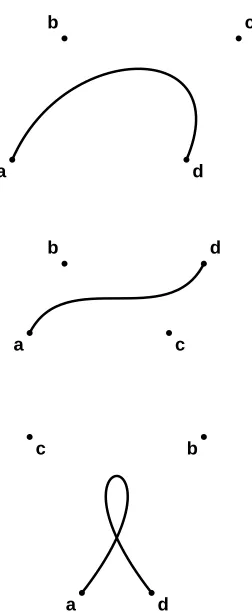
Figure 6. Three B´ezier curves controlled by

a,b,c, andd.

CONGis one of several predefined geometric constraints:

p HOR qconstrains pointspandqto be aligned horizontally,

p VER qconstrains pointspandqto be aligned vertically,

(a,b) CONG (c,d)constrains the distance between the pointsa

andbto equal the distance between the pointscandd, and

(a,b) PARA (c,d)constrains the line through the pointsaandb

to be parallel to the line through the pointscandd.

Figure 7 shows how these constraints can be used to draw a block A. Notice that the segment between two points can be constrained even if it is not painted; the constraints are defined on points, not painted lines.

Constraints are an integral part of the Juno-2 extension language. In general, a Juno-2 command of the form

VAR <var> <hint> IN

<constraint> -> <command> END

has the following operational semantics: introduce a new variable<var>

with a value near<hint>that satisfies<constraint>, then execute

<command>.

Hints are needed to make constraints useful in the face of non-deter-minism. For example, the command

VAR x 1 IN

x * x = 2 -> Print(x) END

prints the positive square root of 2. There are two solutions to the constraint, but the solver will converge on the positive square root, since the hint for

xis positive.

Adjusting. The final step of the standard recipe is to adjust the control points until the picture looks right. There are two tools for moving points in the drawing: theDragtool, which updates the drawing in real time as you move a point; and theAdjusttool, which lets you move a point as an atomic action. Either of these tools can be used to adjust the size, position, and orientation of the equilateral triangle.

a b

c d

e f

g h

i j

k

a HOR b AND a HOR e AND a HOR f AND c HOR d AND j HOR i AND h HOR g AND

(h, a) PARA (b, c) AND (h, a) PARA (b, j) AND (h, a) PARA (b, k) AND (h, a) PARA (b, g) AND (g, f) PARA (e, d) AND (g, f) PARA (e, i) AND (g, f) PARA (e, k) AND (g, f) PARA (e, h) AND (a, b) CONG (c, j) AND (a, h) CONG (g, f) AND (b, c) CONG (j, k)

Figure 7. A block letter A and its associated constraints. The height, width, and thickness of the letter can be changed by dragging.

In the equilateral triangle, as in most figures, the drawing is undercon-strained, so that the solver could move the points by large distances and still satisfy the constraints. If the solver actually did this, the Dragand

the location of the mouse is always used as the hint for the point being moved).

The ability to drag a point while the system continuously solves the constraints and updates the drawing is invaluable, both because it provides a way of making fine aesthetic adjustments, and because it allows motion along a continuous trajectory through the constraint solution space. The latter benefit is especially noticeable in cases where the solution space contains discontinuities. Using theAdjusttool, it is quite easy to inad-vertently flip into another branch of the solution space, but to do so using the drag tool requires a conscious, rapid motion of the mouse.

Most Juno-2 drawings have more than two degrees of freedom, in which case dragging is ambiguous. For example, in many drawings, the constraint solver can accommodate a drag operation either by translating or scaling the drawing, and there is no way to tell which of these the user intends. To ensure that dragging has the intended result, you can freeze the points of the drawing that you want to fix. For example, to adjust the height of the block A in Figure 7 without changing its width or thickness, you could freeze the pointsa,b, andf, and drag eithergorh. You can move the mouse both vertically and horizontally, but because of the constraints,

gandhwill move only vertically.

3

Templates and folding

Most large drawings have repeated elements. It would be too tedious to draw each instance of the repeated element individually; so we produce a template once and instantiate it several times.

Because Juno-2 is programmable, it is possible to define the template by typing the definition of a Juno-2 procedure into the program view. A tool will appear for it in the palette for the module in which it is defined, and the tool can then be used to instantiate the procedure, just as for a built-in tool. For example, the procedures for drawing circular arcs, arrows, and dashed lines are all available as tools in the appropriate palettes.

In many cases a repeated element is simple enough that you can program the template for it by simply drawing the repeated element and folding it into an appropriate procedure. This allows complicated drawings to be produced entirely in the drawing view, without explicit editing in the program view. The folding operation is similar to the grouping and copying operations supported by many drawing programs, but is more general.

VAR

a ~ (203, 505), b ~ (319, 505) IN

a HOR b -> EqTr(a, b); EqTr(b, a) END

a b

Figure 8. Drawing a diamond withEqTr. The equilateral triangle is a simple example of a drawing that you might

want to fold into a procedure. To do this, you draw the triangle as described above, click theFoldbutton, and then specify which of the points are to be parameters to the procedure; the other points become local variables. When you create a new procedure by folding, you supply a meaningful name, for example,EqTr. A new tool appears in the tool palette that can be used just like any of the built-in tools. For example, Figure 8 shows a diamond drawn by two applications ofEqTr.

When a drawing is folded into a procedure, it is critical that the points

that become local variables receive appropriate hints. For example, the drawing of the diamond in Figure 8 depends on the fact thatEqTr(a,b)

draws an equilateral triangle to the left of the rayab. To achieve this, the hint forcmust be to the left of that ray. Since the positions ofaandbvary from call to call, no absolute hint forcwill do. Therefore, before folding the procedure, you must changec’s hint so that it is computed relative to

aandb, instead of absolutely.

Juno-2’sRELfunction is useful for such hints. Ifaandbare points andxandyare real numbers, then the expression

(x,y) REL (a,b)

is the point with coordinates(x,y)in the coordinate system in whichais the origin andbis at the tip of the unitxvector, as shown in Figure 9. For

example,(0.5,0) REL (a,b)is the midpoint of the segmentab. The

RELfunction has the nice property that it is invariant under translation, rotation, and scaling.

a

b (1,0) REL (a,b)

(1,1) REL (a,b) (0,1) REL (a,b)

Figure 9. TheRELfunction.

It is so common to express one point’s hint relative to the location of two other points that a Rel tool is built into the Juno-2 user interface. Applying this tool to the pointsc,a, andbin Figure 5 changes the hints in the program view to the following:

VAR

a (179.5, 197.1),

b (271.2, 223.6),

c (0.5, 0.866) REL (a, b)

IN ... END

TheReltool chooses the numbers in the hint forcbased on the current position ofcrelative toaandb, so the drawing view doesn’t change. The

Reltool has made the command suitable for folding into a procedure with argumentsaandband local variablec.

4

Juno-2 extensibility

The features described so far all derive from Juno-1. In the rest of the report, we describe Juno-2’s powerful extension features, and we present some examples that exploit them.

The Juno-2 programming language is a full-fledged imperative pro-gramming language with conditionals, loops, assignments, global vari-ables, local varivari-ables, procedures, and closures. For example, Figure 10 was produced with a recursive procedure. The drawing operations are those

Figure 10. A dragon curve of order 10. This is an example of a figure drawn by a recursive procedure.

of PostScript [1], and the control structures are those of guarded commands [5, 15]. Larger Juno-2 programs are organized into modules, which are collections of definitions.

ordered pairs is significant. As in pure Lisp [10], they have the virtue of providing structure to the value space sufficient to construct a variety of data structures, including two and three dimensional points, lists, records, and trees. Ordered pairs are allowed in constraints, so it is possible to constrain the structure of a value and to place constraints on its embedded values.

Definitions. Here is the Juno-2 syntax for defining procedures, predi-cates, and functions:

PROC P(<args>) IS <command> END; PRED Q(<args>) IS <constraint> END;

FUNC <res> = F(<args>) IS <constraint> END;

Procedures are parametrized commands; predicates and functions are parametrized constraints. In a function definition, the constraint should determine<res>uniquely from<args>, but Juno-2 doesn’t check this. In a procedure definition, Juno-2 allowsIN,OUT, andINOUTparameters, but in this report we considerINparameters only.

Juno-2 constraints allow existential quantifiers, with the syntax:

(E <var> <hint> :: <constraint>)

This constraint is true if the constraint solver can find a value for the existentially quantified variable (using the optional hint) that makes the constraint true.

For example, here are two simple definitions:

PRED Hor(a,b) IS

(E ax, bx, y :: a = (ax,y) AND b = (bx,y)) END;

FUNC y = Sqrt(x) IS y 1 AND y * y = x

END;

The existentially quantified variables inHorneed no hints, since they are determined by pair constraints and equalities; there is nothing non-linear about them. The result variable forSqrtdoes need a hint, to exclude the negative root.

a

ab

bc

c

d _cd

bcd p = abcd

b

abc

Figure 11. A geometric visualization of the OnBezier predicate with t = 2=3.

This method of constructing a B´ezier curve is known as the de Casteljau algorithm.

As another example, here is a definition of the constraint that the point

plies on the B´ezier curve determined bya,b,c, andd(see Figure 11):

PRED OnBezier(p, a, b, c, d) IS

(E t ..., ab, bc, cd, abc, bcd, abcd

:: ab = (t, 0) REL (a, b) AND bc = (t, 0) REL (b, c) AND cd = (t, 0) REL (c, d) AND abc = (t, 0) REL (ab, bc) AND bcd = (t, 0) REL (bc, cd) AND abcd = (t, 0) REL (abc, bcd) AND p = abcd)

a b c d e f g h i j k l m a b c d e f _g h i j k l m a b c d e f _g h i j k l m

g = NearMid(a, m) g = NearMid(b, l) g = NearMid(c, k) g = NearMid(d, j) g = NearMid(e, i) g = NearMid(f, h) (c, d) PARA (c, e)

Figure 12. Our freehand S is on the left. The sixNearMidconstraints produced the symmetrical but cuspy version in the mid-dle. Adding the PARAconstraint removed the cusps atdandj. Adjusting to taste pro-duced the smooth version on the right.

END

It is well known that fort =1=2, pis the midpoint of the B´ezier cubic.

More generally, p varies over the whole curve as tvaries over the real line. Farin’s text [6] describes B´ezier curves and other models for curves and surfaces. Juno-2’s constraint solver is powerful enough to use this definition effectively, and it is one of Juno-2’s predefined predicates (as are

HorandSqrt). However, theOnBezierpredicate doesn’t work very well unless it has a good initial hint fort, and the formula we use for this hint is complicated enough that we have replaced it by an ellipsis in the listing above.

5

Drawing an S

Drawing an S from scratch is a hard test for any drawing program. Our solution illustrates the value of Juno-2’s programmability.

We started by drawing a rough sketch of the S from four B´ezier curves, as shown first in Figure 12. Next, we used constraints to make the S prettier. We could have made the S radially symmetric about its center pointg, but the top of an S should be smaller than the bottom. So what is really needed is some kind of scaled radial symmetry. Juno-2 provides no predefined constraint for scaled radial symmetry, so we typed the following function definition into the program view:

FUNC mid = NearMid(a,b) IS mid = (0.45, 0) REL (a,b) END;

which caused aNearMidtool to appear. We applied this tool six times to produce the constrained S shown second in Figure 12. To remove the cusps at the pointsdandj, we madec,d, andecollinear by applying a single

PARAconstraint (by symmetry, this also madei, j, andkcollinear). A little dragging produced the final S path.

,

a, b, c, d

PenStroke(

p, q)

trajectory pen

Figure 13 illustrates how the stroke is filled. The pointsa,b,c, and

dcontrol the path of the center of the pen; the tips of the arrows through these points control the path of the right edge of the pen; and the tails of the arrows control the path of the left edge of the pen. Thus it is straightforward to compute these two paths and fill the region enclosed by them. This can still leave a triangular notch to be filled. OurPenStrokeprocedure uses the constraint solver to compute the vertices of the notch: one vertex is on both B´ezier curves, and the others are on the common tangent to the two curves.

a

b

c d p

q

Figure 13. Stroking a calligraphic pen de-fined by the pointspandqover the B´ezier curve a, b, c, d. Arrows are used in the diagram to indicate vectors that are equal.

6

Modules

The Juno-2 language includes modules, to provide organized libraries for common drawing operations. For example, there is a Dashmodule for drawing dashed lines that was used to draw Figure 9. Dash is one of Juno-2’s several dozen predefined modules; the “Open Module” menu in Figure 5 shows the names of most of them. Opening a module gives a menu containing tools for its procedures, predicates, and functions. For example, Figure 5 shows the menu for thePSmodule.

One of the predefined modules is DiGraph, which can be used to draw directed graphs with labeled nodes connected by arrows. The module exports a procedure for drawing a node at a particular point, and for drawing straight or curved edges between nodes. Figure 14 shows the modules imported directly and indirectly into the implementation of theDiGraph

module. The figure was drawn in a few minutes with theDiGraphmodule itself.

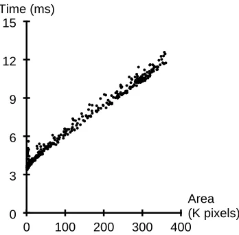
We have also written aPlotmodule for drawing scatter-plots. Fig-ure 15 shows a graph drawn with this module. The graph shows the per-formance of Juno-2’s software double-buffering. The perper-formance section below describes the system configuration on which this data was collected. ThePlotmodule illustrates the use of lists: one of the parameters to the plotting procedure is the list of(x;y)data points to plot.

7

The constraint solver

DiGraph

PS Geometry Arrow Ellipse

Math R2

Figure 14. TheDiGraphmodule and its imports. TheDiGraphmodule itself was used to draw the figure.

The remainder of the report discusses important implementation aspects of the Juno-2 system. Juno-2 consists of a compiler, an interpreter for a virtual machine, and user interface code. The compiler transforms a Juno-2 command into instructions for the virtual machine, which is a bytecode interpreter. TheSOLVEbytecode instruction invokes the runtime constraint solver. In this section, we outline the method used by Juno-2 to solve constraints.

The input to the solver is a list of unknowns to be solved for and a constraint to be solved. In Juno-2, a constraint is a restricted form of

predicate from the first-order theory of the real numbers (with equality) together with the theory of ordered pairs. Constraints may involve ex-istential quantification and conjunction, but not universal quantification, disjunction, or negation. The atomic formulas in constraints may include primitive, predefined, or user-defined predicates or functions (including pair, addition, multiplication, trigonometric, and exponential functions), but not inequalities and integer functions such asFLOORandMOD.

Although we don’t allow inequalities in constraints, we have rarely missed them. Inequality constraints are most useful in systems like user interface toolkits where the system must lay out objects in response to dynamic user input. In Juno-2, we have found that hints give the user more precise control over layout.

However, we have needed inequalities occasionally, for example, to construct sliders. Inequalities can be defined in terms of the built-in Juno-2 primitives. For example,

PRED NonNegative(x) IS (E y :: y * y = x) END; PRED NonZero(x) IS (E y :: y * x = 1) END; PRED Greater(x, y) IS

NonNegative(x-y) AND NonZero(x-y) END;

Unfortunately, the constraint solver doesn’t work very reliably with in-equalities defined in this way. Therefore, to avoid misleading users, we

decided not to predefine them. 0 100 200 300 400

0 3 6 9 12 15

Area (K pixels) Time (ms)

Figure 15. Performance of Juno-2’s soft-ware double-buffering during dragging of a simple drawing. Each point (x;y)

corre-sponds to a single frame; x is the

num-ber of pixels painted for the frame and y

is the elapsed time in milliseconds between that frame and the next. The graph shows that software double-buffering costs about 3 ms / frame plus 1 ms / 40K pixels / frame.

Preprocessing. To reduce the number of unknowns that the solver must handle, the Juno-2 compiler preprocesses the constraints to generate in-line assignments where possible. Extracting these assignments is a limited form of the local propagation technique used by many simple constraint solvers. For example, in the command

VAR x, y, z, w IN x = a + a AND x = y * y AND w = x * a AND z = (x, y) -> ...

which solves for the unknownsx,y,z, andwin terms of the known value

a, the compiler will find pre-assignments forxandw, but will need to rely on the constraint solver foryandz. The resulting instructions are:

x := a + a; w := x * a;

SOLVE(y, z: x = y * y AND z = (x, y))

The compiler could extract post-assignments as well, though it doesn’t do this now. For example, in the example above, the compiler could remove

zfrom the call toSOLVE, inserting an explicit assignment tozafter the call.

Unpacking constraints. After preprocessing, the compiler converts the remaining constraint into a conjunction of primitive constraints that are known to the runtime solver. This process is called unpacking.

Most things that appear to the Juno-2 user to be primitive are actually predefined entities in the Juno-2 language, and are not primitive from the point of view of the constraint solver. For example, while the geometric predicates are built into the user interface, they are not built into the solver: They are defined in terms of addition, multiplication, and pair constraints. Even subtraction and division are predefined. In fact, when all the defini-tions are eliminated, the constraint solver is presented with a conjunction of primitive constraints, of which there are only six types:

FUNC res = SegLenSq(s) IS (E px, py, qx, qy, dx, dy :: s = ((px, py), (qx, qy)) AND qx = px + dx AND

qy = py + dy AND

res = dx * dx + dy * dy) END;

PRED CONG(s, t) IS

SegLenSq(s) = SegLenSq(t) END;

Figure 16. The CONG constraint is not primitive from the point of view of the solver, but is predefined by the Juno-2 definitions above.

x = y x = tan(y) x = y + z x = exp(y) x = y * z x = (y, z)

In these six forms,x,y, andzare variables or constants.

By converting constraints into conjunctions of primitives, we simplify the interface to the runtime solver. Although the number of primitive constraints is small, they are extremely expressive when combined with declarative predicate and function definitions. For example, they can be used to define any constraint expressible in Euclidean geometry. Figure 16 shows the definition ofCONG.

To unpack, the compiler repeatedly replaces predicates and functions with their instantiated definitions and un-nests the term structure by insert-ing existentially quantified variables. For example, given

FUNC y = Half(x) IS x = y + y END

the constraint

u = Half(w * z)

would unpack to

(E s :: s = w * z AND s = u + u)

a b c

VAR

a = (200, 210), b = (300, 310), c ~ (131.6, 333.8) IN

(a, b) CONG (a, c) -> Circle.Draw(a, b); PS.Stroke()

END

Figure 17. The pointcis constrained by a singleCONGconstraint to be on the circle defined by the frozen pointsaandb.

Unpacking interacts with preprocessing, since the replacement of a defined function or predicate with its body can allow new pre-assignments to be extracted. The processes eventually terminate, leaving a list of unknowns and primitive constraints that the compiler bundles together into aSOLVEinstruction for the virtual machine. Figure 18 shows the result of preprocessing and unpacking the command shown in Figure 17 using the definition ofCONGfrom Figure 16. Notice how a pre-assignment was generated for the expressionSegLenSq(seg1)once theCONGpredicate was instantiated.

Separating constraints. The first step in solving a constraint at runtime is to separate the pair and equality constraints from the numeric constraints, so that they can be solved independently. It is intuitively clear that this sepa-ration is possible, since a constraint likex=(y,z)constrains the structure of the solution, while constraints like x=y+z andx=y*z constrain the numeric values embedded in the solution.

Our technique for separating out the pair constraints is based on a technique used in mechanical theorem proving [13].

Unification closure. We use unification closure to solve the pair con-straints. Computing the unification closure is a basic step in resolution theorem-proving and in the type-inference algorithm used by the program-ming language ML.

The input constraint is first converted into a representation called an equivalence graph, or E-graph. An E-graph is a directed graph together with an equivalence relation on its nodes. The nodes of the graph are labeled by variables and function names, and there are ordered edges from each function node to the nodes representing its arguments. Two nodes

a := (200, 210); b := (300, 310); seg1 := (a, b);

seg1LenSq := SegLenSq(seg1); c := (133.5, 247.4);

seg2 := (a, c); SOLVE(

c, seg2, p, q, px, py, qx, qy, dx, dy, dxSq, dySq : seg2 = (a, c) AND seg2 = (p, q) AND p = (px, py) AND q = (qx, qy) AND qx = px + dx AND qy = py + dy AND dxSq = dx * dx AND dySq = dy * dy AND

seg1LenSq = dxSq + dySq); Circle.Draw(a, b);

PS.Stroke()

Figure 18. The command produced by preprocessing and unpacking the command of Figure 17 using the definition for CONG

shown in Figure 16.

are in the same equivalence class if and only if the values they denote must be equal to satisfy the constraint. Initially, each node is in its own equivalence class. Then, for each equality in the input constraint, the equivalence classes of the nodes representing the two sides of the equality are merged.

To solve the pair constraints, the solver computes the unification closure of the E-graph over the pair nodes. This is the smallest equivalence relation such that if pair nodes(x;y)and(x

0 ;y

0

)are equivalent, thenxis equivalent

tox 0

andyis equivalent toy 0

.

In the example shown in Figure 18, unification closure produces four nontrivial equivalence classes. Since the pointsaandbare both frozen, the variables seg1 and seg1LenSq are fixed as well. (Notice that neither occurs in the list ofSOLVEunknowns.) Due to the two constraints involvingseg2, the value forais unified with the variablep. This causes

pxandpyto be unified with the values200and210, respectively. Finally, the unknowncis unified with the unknownq.

The numeric constraints that remain can be considered to constrain the values of equivalence classes in the E-graph, instead of single nodes. The solver exploits this fact to reduce the number of numeric unknowns. Figure 19 shows the numeric constraint system that remains after the pair

SOLVE(

px, py, qx, qy, dx, dy, dxSq, dySq, : qx = 200 + dx AND qy = 210 + dy AND dxSq = dx * dx AND dySq = dy * dy AND 20000 = dxSq + dySq)

Figure 19. The numeric constraint system that remains after applying unification closure to theSOLVEcommand of Figure 18.

constraints have been eliminated from theSOLVEconstraint of Figure 18 by unification closure. Once the numeric solve completes, the unification closure machinery must still construct values for pair-valued unknowns from the numeric values. In this case, the value forcwill be constructed by pairingqxwithqy.

Repacking. One more step is used to reduce the number of unknowns: the primitive numeric constraints and unknowns are repacked. For exam-ple, consider the following three primitive equations in three unknowns:

x = y + 1 z = y * x z = x + 2

Repacking will produce one equation in one unknown:

(x - 1) * x = x + 2

After this equation is solved for x, values foryand zcan be computed immediately. As another example, repacking the constraint of Figure 19 produces one equation in two unknowns:

20000=(qx 200)

2

+(qy 210)

2

Numeric solving. After repacking, the numeric constraints are solved by Newton’s method. This method consists simply in repeating the following step: replace the constraints by the linear constraints that approximate them around the current point, then solve the linear constraints by Gaussian elimination to produce the next point. For an accessible description, see Conte and de Boor’s text [4].

It was not obvious at the start of the project whether Newton’s method would do the trick. Our first version of the solver failed so often that it was unwise to demonstrate it, much less use it. After fixing many problems the solver still is not perfect, but it works well enough to be quite useful. The detailed account of our struggles with Newton’s method belongs in a separate paper, but we will briefly mention the four main problems that needed fixing.

First, hints were lost as the constraints were preprocessed, unpacked, separated, subjected to unification closure, and repacked. We found that each of these steps must be implemented carefully to preserve the informa-tion in the hints. For example, a hinted variable should never be eliminated during repacking unless its hint can be transferred to one of the variables that remain.

Second, we found that ordinary Newton iteration is too willing to move large distances. Because of this, the adjust and drag tools often surprised users by changing the drawing more than necessary to solve the constraints. We fixed this by ensuring that each Newton step was as short as possible.

Third, ordinary Newton iteration is unreliable when the constraints are consistent but redundant. Consistent but redundant nonlinear systems tend to produce inconsistent or ill-conditioned linear systems for the individual steps. To solve this problem, we modified our Gaussian elimination routine to use only the “well-conditioned part” of its matrix and ignore the ill-conditioned part.

Fourth, it is difficult to know when to stop the Newton iteration. Be-cause roundoff errors can occur in unpredictable ways when evaluating the constraints, fixed error thresholds do not work, regardless of whether

they are absolute or relative. We therefore determine the error threshold by estimating the roundoff error.

Why unpack/repack? It seems odd to unpack and later repack. But unpacking is necessary to separate the numeric from the non-numeric con-straints, and repacking makes Newton’s method faster and more reliable. The whole process distills the essential numeric problem out of a large collection of user-defined constraints.

For example, consider the problem of solving the constraint

OnBezier(p, a, b, c, d) -> ...

forp. When all the definitions are unpacked, the result is a conjunction of 99 primitive constraints on 137 unknowns: 39 pair constraints, 36 addition constraints, and 24 multiplication constraints. The compiler finds pre-assignments for 3 of the unknowns, leaving 134; after unification closure, 61 numeric unknowns remain. Fifty-four of these unknowns are eliminated by repacking, so that the final Newton iteration solves a system with six nonlinear constraints on seven unknowns. Without repacking, Newton’s method would have to solve a system of size 61 by 60 instead of 7 by 6. The number of Newton iterations required to solve the system depends on the values ofa,b,c, anddand on the hint forp, but is typically less than five.

8

Performance

In this section we report the performance measurements we have made, and our tentative conclusions about the performance limits of the Juno-2 approach.

4.0

0.5

Figure 20. An engineering-style drawing of a flange and its cutaway view.

The results in this section describe Juno-2 running on a DEC 3000/600 Alpha workstation equipped with a 175 megahertz DECchip 21064 pro-cessor running OSF/1. The entire system is written in Modula-3 [16]. Juno-2’s user interface is based on the FormsVBT [3] and Trestle [11] object-oriented user interface toolkits, which use the X window system [17] for doing graphics. A standard Trestle module provides software double-buffering. Trestle reduces curved paths to polygonal paths; X strokes and fills the polygonal paths.

The reported times include Modula-3 runtime checks and garbage col-lection. We have tuned the program to make the collection costs almost negligible (less than 1.5 per cent of the frame times), but the costs of runtime checks are more significant.

As samples for study, we take three rather simple drawings, the filled equilateral triangle, the block A, and the tetrahedron shown in Figures 5, 7, and 1; and one more complicated drawing, the engineering drawing of the flange shown in Figure 20. We wrote Juno programs to animate these figures, and then measured their per-frame costs.

Per-frame elapsed times for the triangle, block A, and tetrahedron are 16, 40, and 73 milliseconds, respectively. This is fast enough to produce the illusion of continuous motion. The costs in executing each frame can be divided into four categories:

executing the graphics operations to paint the new frame, including

stroking, filling, painting text, communicating with the X server, and the pixmap copy required by software double-buffering,

solving the pair constraints (unification closure), repacking and solving the numerical constraints, and

all other overhead in the bytecode interpreter, including the time to

decode the arguments to the run-time constraint solver.

Figure 21 shows these costs for the triangle, block A, and tetrahedron. The costs of solving the pair constraints are quite significant (more so than the figure indicates, since much of the overhead is attributable to decoding the pair constraints). We estimate that most frame rates will double when we move the pair-solving to compile time.

graphics 11 pair solve 2 numeric solve 1 overhead 2

total 16

Equilateral triangle

graphics 12 pair solve 10 numeric solve 10 overhead 8

total 40

Block A

graphics 14 pair solve 26 numeric solve 12

overhead 21

total 73

Tetrahedron

Figure 21. Per-frame elapsed times of three simple figures, in milliseconds.

The cost of each Newton step is the cost of evaluating the Jacobian plus the cost of performing Gaussian elimination. Asymptotically, Gaussian elimination isO(n

3

)while evaluating the Jacobian is onlyO(n

2

). But for

the matrix sizes we currently observe in Juno-2, evaluating the Jacobian takes about half the time. These numeric algorithms have predictable costs; comparing them with the machine’s SPEC rating indicates that we are not getting the performance we should, even allowing for the costs of runtime checks (which are roughly 25% for these algorithms). We don’t yet know why.

In summary, we are confident that the numeric solving could be made considerably faster and that the pair-solving cost and about half the over-head could be eliminated by moving pair-solving to compile time. This would make graphics dominate the other per-frame costs in simple draw-ings like the equilateral triangle, block A, and tetrahedron.

graphics 58 pair solve 136 numeric solve 118

overhead 142

total 454

Figure 22. Per-frame elapsed times of the flange, in milliseconds.

A more important question is how the cost of constraint solving scales. The flange example addresses this question, since it uses many of the pre-defined Juno-2 modules, such as those for drawing circular arcs, dashed lines, and arrows. The per-frame elapsed time for the flange is 454 mil-liseconds (see Figure 22), which is responsive enough to be usable, but not to provide the illusion of continuous motion during dragging or animation. Juno-2 encourages the user to structure a drawing as a hierarchy of groups and subgroups, using defined procedures and predicates, so that drawing a frame involves solving many small systems instead of one big

one. For example, in drawing the flange, the constraint solver is invoked 157 times per frame, but the largest of these 157 systems is only 12 by 12. Thus, in the case of the flange, hierarchy is working. (The reader may be surprised by the number of invocations of the constraint solver. Our style certainly does not spare the constraint solver: it is invoked for each dash of a dashed line and for many circular arcs.)

Of the 157 invocations of the solver per frame of the flange, 105 of them produced trivial matrices (zero by zero). This could easily be fixed by preprocessing more aggressively. Of the 52 nontrivial numeric solves, all of them were square matrices. This is because the process of repacking constraints tends to produce final Newton systems that are square or nearly square. Figures 23 and 24 show histograms illustrating the number of Newton steps required and the sizes of the matrices for these 52 invocations of the solver.

0 5 10 15

1 2 3 4 5 6

Figure 23. Most of the 52 calls to Newton’s method used to draw the flange took 3 or 4 iterations; none took more than 6.

The distribution of the number of Newton iterations in Figure 23 is encouraging. As long as adequate hints are provided, we expect this number to remain near four even for very large drawings. (The spike at one iteration is because some of the systems are actually linear. This could be detected at compile time, but there is no clear advantage in doing so.)

The distribution of the sizes of the Newton systems in Figure 24 is not so encouraging. It is not clear how the matrix size will scale as drawings get larger. Hierarchy helps, but until Juno-like methods see more use, we won’t know how much. To adapt our methods to particular applications, it may be necessary to design the application carefully to keep the matrix sizes manageable.

9

Conclusions

Juno-2 shows that fast constraint solving is possible with a highly extensi-ble, fully declarative constraint language. The Juno-2 constraint language allows first-order function and predicate definitions as well as structural and non-linear constraints. By adding ordered pairs to the theory, we support a variety of structural constraints without greatly complicating the solver.

5 10 15 20 25

1 2 4 6 12

0

Figure 24. The 52 calls to Newton’s method used to draw the flange produced matrix sizes ranging from 1 by 1 to 12 by 12. All the matrices were square.

Juno-2 is structured around a small number of general primitives whose combinations are highly expressive. In Juno-2, as in so many systems, this structure was effective in maximizing functionality and minimizing complexity.

Constraints do not eliminate the need for careful thinking, and it takes practice to use them effectively. But they do remove much of the tedium from graphical programming. A flexible constraint mechanism allows you to specify graphical shapes at a level of abstraction that is close to the artwork itself, avoiding the need for explicit calculations of coordinates.

Using Juno-2 is fun. Our experiments with it have strengthened our belief that constraints are destined to become an important enabling tech-nology in interactive graphics. We hope that some of the techniques explored in Juno-2 will be useful steps towards that future.

Acknowledgments

Andrew Myers implemented the Juno-2 virtual machine and parts of the user interface. Lyle Ramshaw and Dave Detlefs contributed illustrations to Figure 1. We’d also like to thank Cynthia Hibbard and Lyle for comments on drafts of this report, Eric Veach for helpful suggestions about handling consistent but redundant constraints, and Jorge Stolfi for drawing the terrific cartoon on the title page.

References

[1] Adobe Systems Inc. PostScript Language Reference Manual. Addi-son-Wesley, 1985.

[2] Alan Borning. The programming language aspects of ThingLab, a constraint-oriented simulation laboratory. ACM Transactions on

Pro-gramming Languages and Systems v. 3, no. 4, pp. 353–387, 1981.

[3] Gideon Avrahami, Kenneth P. Brooks, and Marc H. Brown. A two-view approach to constructing user interfaces. ACM SIGGRAPH ’89

Conference Proceedings, pp. 137–146, August 1989.

[4] S. D. Conte and Carl de Boor. Elementary Numerical Analysis. McGraw-Hill, 1972.

[5] Edsger W. Dijkstra. A Discipline of Programming. Prentice-Hall, 1976.

[6] Gerald Farin. Curves and Surfaces for Computer Aided Geometric

Design: A Practical Guide, second edition. Academic Press, 1990.

[7] Michael Gleicher and Andrew Witkin. Drawing with constraints. The

Visual Computer, to appear v. 11, no. 1, 1994.

[8] John D. Hobby. A User’s manual for MetaPost. Available via anony-mous FTP as the file162.ps.Zfrom netlib.att.comin the directorynetlib/research/cstr.

[9] Donald E. Knuth. TeX and METAFONT, New Directions in

Typeset-ting. Digital Press and the American Mathematical Society, Bedford,

Massachusetts, 1979.

[10] John McCarthy. Recursive functions of symbolic expressions and their computation by machine. Communications of the ACM, v. 3, no. 4, pp. 184–95, 1960.

[11] Mark S. Manasse and Greg Nelson. Trestle Reference Manual. Re-search Report 68, Digital Systems Reserach Center, 1991.

[12] Brad A. Myers, Dario Giuse, Roger B. Dannenberg, Brad Vander Zanden, David Kosbie, Philippe Marchal, Ed Pervin, Andrew Mick-ish, and John A. Kolojejchick. The Garnet toolkit reference manuals: support for highly-interactive, graphical user interfaces in Lisp. Tech-nical Report CMU-CS-90-117, Carnegie Mellon University, March, 1990.

[13] Greg Nelson. Techniques for program verification. Research report CSL-81-10, Computer Science Laboratory, Xerox Parc, 1981. Section 5.

[14] Greg Nelson. Juno, a constraint-based graphics system. ACM

SIG-GRAPH 85 Conference Proceedings. July, 1985.

[15] Greg Nelson. A generalization of Dijkstra’s calculus. ACM TOPLAS v. 11, pp. 517–61, October 1989.

[16] Greg Nelson, editor. Systems programming with Modula-3. Prentice-Hall, 1991.

[17] Robert W. Scheifler, James Gettys, and Ron Newman. X Window

System 2nd ed. Digital Press, 1990.

[18] Steve Sistare, Graphical interaction techniques in constraint-based geometric modeling, Graphics Interface ’91. 1991.

[19] Ivan Sutherland. Sketchpad, a man-machine graphical communica-tion system. Proceedings of the Spring Joint Computer Conference, pp. 507–524, Detroit, MI, May 21–23, 1963.