101a
The Second Annual Video Review
of Computational Geometry
Edited by Marc H. Brown and John Hershberger
May 4, 1993
d i g i t a l
Systems Research Center
Systems Research Center
The charter of SRC is to advance both the state of knowledge and the state of the art in computer systems. From our establishment in 1984, we have performed basic and applied research to support Digital’s business objectives. Our current work includes exploring distributed personal computing on multiple platforms, network-ing, programming technology, system modelling and management techniques, and selected applications.
Our strategy is to test the technical and practical value of our ideas by building hardware and software prototypes and using them as daily tools. Interesting systems are too complex to be evaluated solely in the abstract; extended use allows us to investigate their properties in depth. This experience is useful in the short term in refining our designs, and invaluable in the long term in advancing our knowledge. Most of the major advances in information systems have come through this strategy, including personal computing, distributed systems, and the Internet.
We also perform complementary work of a more mathematical flavor. Some of it is in established fields of theoretical computer science, such as the analysis of algorithms, computational geometry, and logics of programming. Other work explores new ground motivated by problems that arise in our systems research. We have a strong commitment to communicating our results; exposing and testing our ideas in the research and development communities leads to improved un-derstanding. Our research report series supplements publication in professional journals and conferences. We seek users for our prototype systems among those with whom we have common interests, and we encourage collaboration with uni-versity researchers.
c
Digital Equipment Corporation 1993
The copyright of each section in this report is held by the author of the section. Similarly, the copyright of each segment of the accompanying videotape is held by the contributor of the segment. All other material in the report is copyrighted
c
Digital Equipment Corporation 1993. This work may not be copied or
Abstract
Computational geometry concepts are often easiest to understand visually, in terms of the geometric objects they manipulate. Indeed, most papers in the field rely on diagrams to communicate the intuition behind their results. However, static figures are not always adequate.
Preface
Computational geometry concepts are often easiest to understand visually, in terms of the geometric objects they manipulate. Indeed, most papers in the field rely on diagrams to communicate the intuition behind their results. However, static figures are not always adequate: geometric algorithms are inherently dynamic, and the per-ception of a 3D object is greatly enhanced by the dynamics of “spinning” the object. The accompanying videotape shows advances in the use of algorithm animation, visualization, and interactive computing in the study of computational geometry. The following pages contain brief descriptions of all the segments of the videotape. The eight segments in the video cover a wide range of geometric concepts and software systems.
Although the segments are independent of each other (and, indeed, have been prepared by different authors), a number of themes are evident: The first two seg-ments are animations of fundamental algorithms (Fortune’s sweep-line algorithm for computing a Voronoi diagram, decomposition of 3-D polyhedra). The follow-ing three segments are animations of motion plannfollow-ing algorithms, both in 2-D and in 3-D. Next are two segments showing geometric “workbenches,” both a general purpose workbench and one tailored to the particular domain of range searching. The last segment of the videotape shows a sequence of 3-D objects with some interesting properties.
We thank the members of the Video Program Committee for their help in evaluating the entries. Besides us, the members of the committee were Marshall Bern (Xerox PARC), Michael Kass (Apple), Leo Guibas (DEC SRC/Stanford University), and Jim Ruppert (NASA). We also thank Bob Taylor of the DEC Systems Research Center for his support in publishing the 1st Annual Review last year; it’s available as SRC Research Report #87a (a written guide) and #87b (the videotape) by sending electronic mail [email protected].
We believe that visualization and algorithm animation has a powerful role to play in communicating the ideas of geometric algorithms; the accompanying videotape illustrates some of this power. We hope this video review will inspire others to implement and display their own algorithms and geometric objects, so that “lively” diagrams will become increasingly common in computational geometry.
Table of Contents
Length Title/Author Page
1
7:47 Visualizing Fortune’s Sweepline Algorithm 1 for Planar Voronoi DiagramsSeth Teller
2
6:01 Building and Using Polyhedral Hierarchies 4David Dobkin and Ayellet Tal
3
6:44 Moving a Disc between Polygons 8Stefan Schirra
4
8:29 Compliant Motion in a Simple Polygon 12John Hershberger
5
8:47 Implementation of a Motion Planning System 17 in Three DimensionsEstarose Wolfson and Micha Sharir
6
7:14 Animation of Geometric Algorithms using GeoLab 22P. J. de Rezende and W. R. Jacometti
7
6:02 Ranger: A Tool for Nearest Neighbor Search 27 in High DimensionsMichael Murphy and Steven S. Skiena
8
4:39 Objects That Cannot Be Taken Apart With Two Hands 32Visualizing Fortune’s Sweepline
Algorithm for Planar Voronoi Diagrams
Seth J. Teller
Institute of Computer Science
Hebrew University of Jerusalem
Givat Ram
Jerusalem 91904 Israel
1
The accompanying videotape shows a visualization of Fortune’s sweepline algo-rithm for planar Voronoi diagrams. The algoalgo-rithm sweeps upward through the set of input sites, maintaining a parabolic wavefront consisting of points equidis-tant from the sweepline and the sites. Voronoi edges are traced wherever adja-cent parabolic arcs intersect; Voronoi vertices are left behind wherever an arc is overtaken by its neighbors. In fact, the algorithm computes a transformation of the diagram, in which the wavefront maps to the sweepline itself, and all events (i.e., arc disappearances) occur above the sweepline. Some applications of the Voronoi diagram are demonstrated, including nearest neighbor-finding, Delaunay triangulation, and planar convex hull. Finally, an intriguing connection between
d-dimensional Voronoi diagrams and(d+1)-dimensional convex hulls is depicted
(ford=2).
Visualization
Given a set of sites inddimensions, the Voronoi diagram of the sites is a partition
1
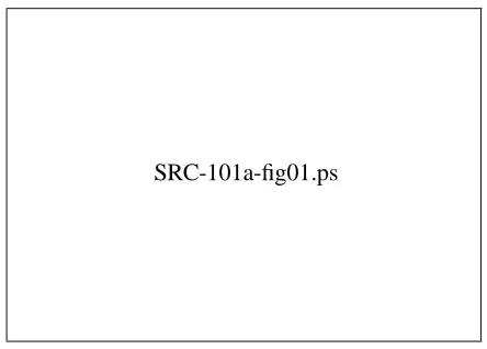
[image:8.612.194.416.132.291.2]SRC-101a-fig01.ps
Figure 1: Fortune’s sweepline algorithm in action.
sweepline algorithm for the construction of planar Voronoi diagrams was presented by Fortune [1]. The sites are first sorted in the direction of sweepline motion. The algorithm then maintains a parabolic wavefront consisting of points equidistant from the set of input sites and the sweepline. Each site encountered by the sweepline contributes one or more sections of an arc to the wavefront. The intersections of adjacent arcs trace the edges of the sites’ Voronoi diagram. When an arc is overtaken by its neighbors, the existence of a triple-point, or point equidistant from three sites, is established and a Voronoi vertex is generated.
The algorithm itself operates discretely, by inferring the presence of each arc disappearance or site, and handling each in turn. Our visualization smoothly animates the evolution of the sweepline between these discrete events. See Fig. 1. Fortune’s algorithm uses a coordinate transformation (the “*-map”) that maps the parabolic wavefront to the sweepline itself. Consequently, all triple-points scheduled by the algorithm occur above the sweepline, where they can be correctly processed. The action of this coordinate transformation on the wavefront, and on the Voronoi diagram, is also depicted in the video.
The videotape demonstrates several applications of the Voronoi diagram. A site’s nearest neighbors are those with which it shares a Voronoi edge. The Delau-nay triangulation is the straight-line dual of the Voronoi diagram. The convex hull of the sites consists of those triangulation edges that occur as part of exactly one triangle.
1
[image:9.612.197.415.133.289.2]SRC-101a-fig02.ps
Figure 2: The first step in illustrating the correspondence between a 2-d Voronoi diagram and a 3-d convex hull.
diagrams and (d +1)-dimensional convex hulls, described by Preparata and
Shamos [2]. Suppose a right paraboloid is erected on the z = 0 plane. Lift
each site to the paraboloid, and consider the tangent plane there, oriented so that its positive halfspace contains the paraboloid (see Fig. 2). The intersection of these positive halfspaces is a polyhedral set whose face structure corresponds to the face structure of the Voronoi diagram.
Acknowledgments
The visualization was produced with graphics hardware and software provided by Silicon Graphics, Inc. The author is grateful to Silicon Graphics for their generous support of this visualization effort.
References
[1] S. Fortune. A sweepline algorithm for Voronoi diagrams. Algorithmica, 2:153– 174, 1987.
Building and Using Polyhedral Hierarchies
David Dobkin
Ayellet Tal
Department of Computer Science
Princeton University
Princeton, NJ 08544
2
The accommpanying videotape shows the techniques used to build a hierarchy of polyhedra as a preprocessing step for intersection detection algorithms. It is an animation of ideas developed in the papers by Dobkin and Kirkpatrick [1, 2]. We show here how the hierarchy is created from a polyhedron and animate an algorithm for detecting the intersection between a polyhedron and a plane.
The Algorithm
The hierarchical data structure gives a concise representation for polyhedra that is useful in various searching tasks. Given a polyhedron,P, we build a hierarchy P0 = P ;P1;:::;P
k such that P
k is a tetrahedron. Each P
i+1 is the convex hull
of a subset of the vertices of its parentP i.
P
i+1 is formed by removing in turn
each vertex inV(P i+1
) V(P i
). The cone of faces attached to the vertex is also
removed. This leaves a hole in the polyhedron. This hole is retriangulated in convex fashion. By removing an independent set of vertices, we assure that the apexes of removed cones are not connected. As a result we can reattach one or many cones and retain a convex object. In Fig. 3 we demonstrate the removal of the cones corresponding to an independent set of vertices. In Fig. 4, new faces are attached to fill in the holes in convex fashion.
2
[image:11.612.194.415.131.307.2]SRC-101a-fig03.ps
Figure 3: Removing an independent set of vertices.
stored in linear space. The initial segment of the video shows the creation of a 6 level hierarchy from a convex polyhedron built on 30 vertices. Colors are used to code the levels .
The hierarchy has been constructed as a search tool. We demonstrate its use in searching during the final segments of the video. We begin with the task of
SRC-101a-fig04.ps
[image:11.612.195.411.436.608.2]2
[image:12.612.196.414.131.305.2]SRC-101a-fig05.ps
Figure 5: Attaching vertex cones that might produce a new closest vertex.
determining if a polyhedron intersects a plane. This is done by determining if the polyhedron at each level of the hierarchy intersects the plane and finding the closest vertex if there is no intersection. At the initial level, this computation can be done in constant time by enumeration. The hierarchy was constructed to simplify growth between levels. In particular, we need only consider growth affecting two
SRC-101a-fig06.ps
[image:12.612.195.414.436.606.2]2
edges adjacent to the closest vertex. This amounts to a maximum of 4 cones reattached at each level. In Fig. 5, we show the cones being attached at a level of growth of the hierarchy, Since the cones are formed from vertices of bounded degree, this growth can be done in constant time, also. As a result, a preprocessed polyhedron’s intersection with a plane can be detected inO (log n)time. We trace
the hierarchical growth by highlighting the closest vertex and extremal edges. We also display the separating plane. Watching the cones return to the polyhedron we are able to see the algorithm determine if a near vertex is closest or new edges are extremal. This case is illustrated in Fig. 6 where an attached vertex punctures the previous plane of support resulting in a new closest vertex.
Acknowledgments
This video was prepared in the computer science department at Princeton Univer-sity. Animation software was attached to code for computing the hierarchy and detecting intersections. The programs were written in C to run under UNIX on a Silicon Graphics Iris. Recording was done at the Interactive Computer Graph-ics Lab at Princeton and editing was done with the assistance of the Princeton Department of Media Services.
We thank Copper Giloth for helping with artistic aspects of the animation. Kirk Alexander and Mike Mills provided superb assistance in producing the final video. This work supported in part by the National Science Foundation under Grant Number CCR90-02352 and by The Geometry Center, University of Minnesota, an STC funded by NSF, DOE, and Minnesota Technology, Inc.
References
[1] D. Dobkin and D. Kirkpatrick, Fast detection of polyhedral intersections,
Journal of Algorithms, 6, 381-392, 1985.
Moving a Disc between Polygons
Stefan Schirra
Max-Planck-Institut f¨ur Informatik
66123 Saarbr¨ucken, Germany
3
The accompanying videotape illustrates a motion planning algorithm developed by Rohnert [5]. The object to be moved is a disc, the obstacles are simple disjoint polygons inside a bounding polygon. We are looking for a collision-free path for the disc between two given positions.
The Algorithm
Rohnert’s algorithm is based on an algorithm by O’D´unlaing and Yap [4] and moves the disc along the Voronoi diagram of the polygons. The set of obstacles is preprocessed such that find path queries in the same polygonal environment can be answered quickly. A find path query fixes the size of the disc, its initial position
pinand its final positionpfi.
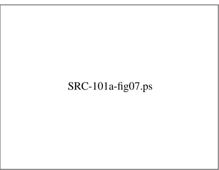
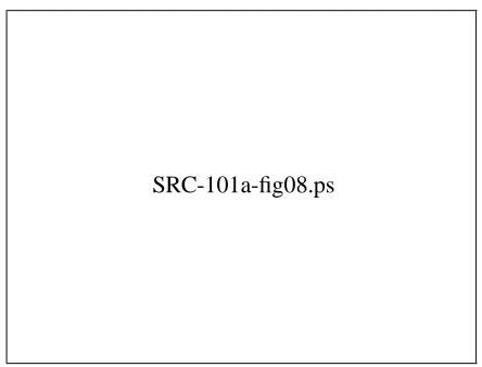
In the preprocessing step the Voronoi diagram of the polygonal environment is computed and a refinement of the planar subdivision given by the Voronoi diagram and the polygons is preprocessed for point location (see Fig. 7). Then a subtree of the Voronoi diagram is constructed that maximizes the sum of the minimum distances on its edges (see Fig. 8). This tree is called MBST. For any two Voronoi vertices the MBST-path connecting them is a safest path (Lemma 4 in [5]). The
MBST is stored in a data structure called edge tree. With this data structure the
bottleneck on a tree path can be found in constant time.
3
[image:15.612.197.414.131.299.2]SRC-101a-fig07.ps
Figure 7: Subdivision defined by polygons and their Voronoi diagram.
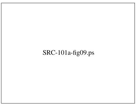
computing v(pin) and v(pfi) the bottleneck on the unique tree path connecting v(pin) and v(pfi) is compared to the size of the query disc. If the bottleneck is
sufficiently large, the algorithm reports a path consisting of a safe path frompinto v(pin), the MBST-path fromv(pin)tov(pfi)and a safe path fromv(pfi)topfi. (See
Fig. 9.) Details of the algorithm can be found elsewhere [5].
Contents of the Video
The video shows collision-free motions computed by the algorithm for several find path queries in three different environments. The construction of the solution paths, especially the construction of a safe path connectingp 2fpin;pfigtov(p),
is illustrated. Furthermore Voronoi diagrams, MBSTs, and refined planar subdi-visions for locating initial and final positions are shown. Note that the Voronoi diagram shown in the video is the intrinsic Voronoi diagram as defined by Yap [6]. Rohnert [5] defines the Voronoi diagram in a slightly different way.
Implementation Notes
3
[image:16.612.194.416.131.300.2]SRC-101a-fig08.ps
Figure 8: MBST – maximum bottleneck spanning tree.
the implementation assumes general position. For point location an algorithm of Edelsbrunner et al. is used [1]. The MBST is computed using Kruskal’s algorithm and Union-Find with path compression and union by rank. In the edge tree data structure a constant-time nearest common ancestor algorithm of Harel and Tarjan is used [2]. Most of the implementation was done in a “Fortgeschrittenenprak-tikum” at Universit¨at des Saarlandes by Thomas Latz, Thomas Lauer, Margit Paul, and Karsten Rech, and the implementation was finished at MPI f¨ur Informatik. Graphical output is based on Xlib. The video is generated by a single C program and was recorded in real time on a SUN SPARCstation with XVideo of Parallax Graphics. “Real time” includes preprocessing time for the polygonal environments and computation time for the motions in the examples.
Acknowledgments
Thanks to Roland Berberich, Wladimir Minenko, and Walter Reinhard for their help in producing the video.
References
3
[image:17.612.195.417.131.301.2]SRC-101a-fig09.ps
Figure 9: No path exists.
[2] D. Harel and R.E. Tarjan. Fast algorithms for finding nearest common ances-tors. SIAM Journal on Computing, 13(2):338–355, 1984.
[3] S. N¨aher and K. Mehlhorn. LEDA — A Library of Efficient Data Types and Algorithms. In Int. Coll. on Automata, Languages and Programming, ICALP
90, LNCS 443, pages 1–5, 1990.
[4] C. O’D´unlaing and C. Yap. A “retraction” method for planning the motion of a disk. Journal of Algorithms, 6:104–111, 1985.
[5] H. Rohnert. Moving a disc between polygons. Algorithmica, 6:182–191, 1991.
[6] C. Yap. An O(nlogn) algorithm for the Voronoi diagram of a set of simple
Compliant Motion in a Simple Polygon
John Hershberger
DEC Systems Research Center
130 Lytton Avenue
Palo Alto, California 94301
4
The accompanying videotape shows an animated version of an algorithm for com-pliant motion planning in a simple polygon. The video illustrates the use of a number of algorithm animation techniques.
Algorithmic Ideas
Compliant motion is a simple model of robot motion: Once the robot starts moving, it always heads in the same direction. When the robot hits an obstacle obliquely, it slides along the obstacle so as to make positive progress in its programmed direction. Fig. 10 shows compliant-motion paths from two different starting points that reach a specified goal point, shown as a red dot. (Although the figures in this video description are printed only in black and white, the text describes them using the colors employed in the videotape.)
The algorithm shown in the video, developed by Friedman, Hershberger, and Snoeyink [3], computes the set (shown in green) of all points from which the robot can reach the goal in a single programmed movement.
For any point, the set of directions in which the robot can reach the goal from that point forms a single angular range. To find these ranges, the algorithm first computes the set of points from which the robot can reach the goal by moving in a particular fixed direction. It then maintains the set while rotating the direction
through 360
4
[image:19.612.184.428.132.301.2]SRC-101a-fig10.ps
Figure 10: An example of compliant motion.
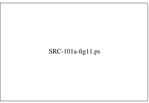
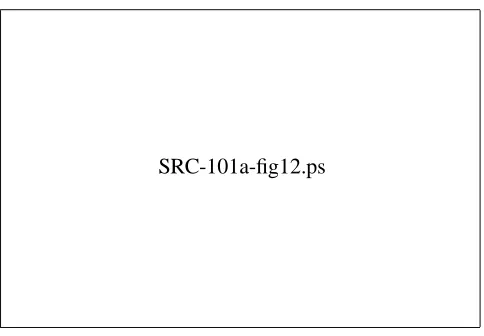
angular range. When a point enters the set, it is added to a start subdivision; when it leaves, it is added to a stop subdivision, as shown in Fig. 11. Color encodes the directions at which points are added to the two subdivisions, and hence records the history of the algorithm. The pink region in the top right view is the current set of points—points already in the start subdivision, but not yet in the stop subdivision. After the two subdivisions are completed, the user can specify an initial robot position with the mouse, as in Fig. 12. In response to the query, the algorithm locates the point in the two subdivisions (the results are highlighted in green), combines the results to get the range of feasible directions (the black angle in the upper-right view), and computes the robot’s path (highlighted in purple).
Animation Techniques
This section itemizes some of the algorithm animation techniques used in the videotape. For more details on techniques see Brown and Hershberger [2].
Multiple views. It is generally more effective to illustrate an algorithm with
4
[image:20.612.185.427.131.298.2]SRC-101a-fig11.ps
Figure 11: Building the start and stop subdivisions.
relationship between color and direction. This relationship is then used in the “Rainbow Start” and “Rainbow Stop” views to emphasize the directions associated with regions in the two subdivisions.
State cues. Changes in the state of an algorithm’s data structures are reflected
on the screen by changes in their graphical representations. As the compliant motion algorithm rotates through 360
, the “Alpha” view pivots an arrow, and the region of points from which a robot can reach the goal by moving in direction
(the-backprojection) pivots with the arrow. Trapezoidal regions are added to
the start and stop subdivisions in response to the algorithm’s actions.
The animation uses color to reflect the algorithm’s state. In the “Both (Angle)” view (so-called because it contains information from both the start and stop sub-divisions), points in the polygon interior change from gray to pink when they are added to the start subdivision. When they are added to the stop subdivision, they change color to green. Thus the current-backprojection is always shown in pink,
and the final non-directional backprojection (the region from which it is possible for a robot to reach the goal by moving in some direction) is painted green at the end of the algorithm. In the “Parallel Start” and “Parallel Stop” views, the two subdivisions, which are otherwise similar in appearance, are distinguished by pink and light blue coloring.
Static history. It is often helpful to present a static view of the history of an
4
[image:21.612.185.427.131.299.2]SRC-101a-fig12.ps
Figure 12: Using the subdivisions to plan a motion.
the start or stop subdivision is graphically labeled with the directionat which it
was added to the subdivision. Since the algorithm rotatesmonotonically, color
also indicates the time order of addition.
Amount of input data. It is important to introduce an animation of an unfamiliar
algorithm on a small problem instance. The video presents the details of the compliant motion algorithm by walking through a small example (Fig. 12). It finishes by reinforcing the ideas of the small example on a larger polygon (Fig. 11).
Highlighting. The key events of the algorithm are associated with vertices and
edges of the polygon. The animation focuses attention on those key vertices and edges by temporarily painting them with a transparent, contrasting purple color. The highlight color draws the eye to the data elements without hiding them. A second use of highlighting is to display transient computations without permanently altering the on-screen state. The robot paths of Figs. 10 and 12 are drawn only in highlighting, since they don’t change the underlying data structures.
Implementation Notes
This animation was produced using the Zeus system for algorithm animation [1]. Zeus has recently been ported to Modula-3, which runs on a variety of X worksta-tions. Modula-3 is available via anonymous FTP fromgatekeeper.dec.com
4
animations are part of the standard Modula-3 distribution.
The most up-to-date information about Modula-3 can be found in the Usenet newsgroupcomp.lang.modula3. If you do not have access to Usenet, there is a relay mailing list; send a message [email protected] to be added to it.
References
[1] M. H. Brown. Zeus: A system for algorithm animation. In Proc. 1991 IEEE
Workshop on Visual Languages, October 1991.
[2] M. H. Brown and J. Hershberger. Color and sound in algorithm animation.
IEEE Computer, 25(12):52–63, December 1992.
[3] J. Friedman, J. Hershberger, and J. Snoeyink. Compliant motion in a sim-ple polygon. In Proceedings of the 5th ACM Symposium on Computational
Implementation of a Motion Planning System in
Three Dimensions
Estarose Wolfson and Micha Sharir
Robotics Laboratory
Courant Institute of Mathematical Sciences
New York University
5
The accompanying videotape depicts motion planning for a point robot moving in a fixed environment of 3 dimensional polyhedral obstacles. It displays graphically the output of a motion planning system that has been implemented at the Robotics Laboratory of the Courant Institute of Mathematical Sciences, New York University. The implemented system is the first version of a planned system that will aim to implement efficient motion planning algorithms for a rigid object translating in 3-space in a similar polyhedral environment (where we plan to exploit the recent theoretical progress made on this problem in [1]). The system is implemented using a combinatorial algorithmic approach, and aims to achieve efficient worst-case performance, while also being fast in practice. It constructs a cell decomposition of the given environment, and uses it to obtain a discrete representation (“connectivity graph”) of free space, which is then used for planning paths between any pair of specified initial and final system placements. The method bears some similarities to a recent technique of Chazelle and Palios [2], but differs from it in many aspects.
The System
5
[image:24.612.128.488.137.508.2]SRC-101a-fig13.ps
Figure 13: Upper left: A view of the polyhedral environment consisting of 21
5
[image:25.612.129.485.134.490.2]SRC-101a-fig14.ps
Figure 14: Upper left: A perspective view from the robot as it traverses the
space along the generated path. The black and green bars represent the vertical boundary of the current cell through which the robot is passing. Upper right: A snapshot of a more complex path and the set of cells it still has to traverse. The path’s route from the center of a common wall is quite visible here. Lower left: Another ride on the robot through space along a different path, showing another cell it currently traverses. In this example there are 392 cells in the environment decomposition, which were generated in 5 seconds on a SUN Sparc II workstation.
Lower right: A snapshot of the path and the set of cells it still has to traverse at the
5
directly above and below the edge are met; we refer to the intersections of such a wall with these next obstacles as etchings). Here a reflex edge is defined as an edge e whose two adjacent faces lie on the same side of the vertical plane
passing throughe (this restricted definition of reflex edges excludes in practice
most concave edges of free space and thus makes the system construct far fewer cells than would otherwise be required). These reflex edges form the so-called
silhouettes of the obstacles. The erected walls may of course intersect each other
(at so-called critical silhouette points), and together they partition the free space into vertical prism-like cells, whose top and bottom boundaries, however, may consist of many faces, but at any rate they arexy-monotone (pieces of so-called
“polyhedral terrains”). Thexy-projection of a cell need not be convex, though,
and a second decomposition step splits cells further so as to obtain cells with convex xy-projections. The program then determines adjacency of cells across
vertical walls, and constructs a “connectivity-graph” to represent this adjacency of cells. Finally, the program selects a center point in each cell, and an exit/entry center point on each vertical wall boundary between pairs of adjacent cells, and constructs canonical paths from the cell-center point to each exit point (roughly speaking, these paths are drawn mid-way between the floor and ceiling of the cell). Given initial and final placements of the robot, the program then locates the cells containing these placements, determines that these cells are reachable from each other via a path in the connectivity graph (or else reports that no free path connecting the initial and final placements exists), finds paths connecting each of these placements to the center of the corresponding cell, and combines these paths with a sequence of pre-stored paths which connect between these cells, to obtain the desired path between the given placements. The reader is referred to [3] for more details concerning the system.
The Videotape
5
equipment is available at the NYU Robotics Laboratory and the Courant Institute. Audio was added separately on local equipment.
The basics of the algorithm are explained with a simple environment containing 2 boxes, one inside the other. For this situation, we see the silhouettes, the critical points, the etchings of walls on other surfaces, the construction of cell walls between the reflex edges and the etchings, the first level of cells, the further decomposition of the cells into subcells with convexxy-projections, and the final resulting cells. We
display each of the 10 final cells of the decomposition. Then we pick 2 points, gen-erate a path between them, and show the sequence of cells that this path traverses. We then ride the robot through the environment along the path, showing each cell as we traverse it. Next the animation turns to the complex environment of 21 obsta-cles, showing the motion planning for 4 consecutive pairs of ‘query’ placements. We show the environment, the silhouettes, and, for each pair of source and destina-tion placements, the generated path and its corresponding sequence of cells. The final segment shows the ride on the robot through the environment, simultaneously displaying the cell we are presently within, moving along a trajectory constructed by linking the 4 paths together. Since the paths computed by the algorithm are polygonal, the ride on the robot tends to be ‘jerky’ as it turns sharply at path cor-ners. An attempt is made to smooth the displayed ride by continuously changing the viewing direction along each path edge, so as to make it continuous at each turn.
Acknowledgments
Thanks to Ed Friedman of the Academic Computing Facility at NYU’s Courant Institute, Rajesh Raichoudhury of the Graphics Lab in the Robotics Lab, and Manfred Mohr, artist, for help and assistance with the video equipment and editing.
References
[1] B. Aronov and M. Sharir, Castles in the air revisited, Proc. 8th ACM Symp.
on Computational Geometry (1992), 146–156.
[2] B. Chazelle and L. Palios, Triangulating a nonconvex polytope, Discrete
Comput. Geom. 5 (1990) 505–526.
Animation of Geometric Algorithms using
GeoLab
P. J. de Rezende
W. R. Jacometti
Departamento de Ciˆencia da Computac¸˜ao
Universidade Estadual de Campinas
13081-970 Campinas, SP, Brazil
6
The accompanying videotape presents two animation modes provided by the geo-metric laboratory GeoLab which we have developed as a programming environ-ment for impleenviron-mentation, testing and animation of geometric algorithms. GeoLab runs on SparcStations under Sun/OS using the XView graphics library, following the OpenLook graphical user interface guidelines.
Introduction
The need for programming environments for the development of geometric algo-rithms has been evident for more than a decade. The intricacy of many solutions to problems that dwell in the realm of computational geometry calls for the com-pilation of several resources into a single programming environment.
6
[image:29.612.196.416.131.335.2]SRC-101a-fig15.ps
Figure 15: Facilities offered by the GeoLab system.
recently Zeus [3], Stasko’s Xtango [9] and de Rezende and Amorim’s AnımA [1] are witnesses to this fact.
The Geometric Laboratory GeoLab
GeoLab [5] as an environment for development of geometric algorithms relates
to the ones mentioned above in the sense that its goal is to aid in the process of software production (specifically in computational geometry), by providing fundamental data structures and algorithms as well as mechanisms that ease the implementation of many desirable features. In a nutshell, GeoLab consists of:
A graphical and interactive programming environment for the manipulation
of geometric models;
Mechanisms for the inclusion of (dynamically linked) new algorithms and
external geometric objects;
6
[image:30.612.196.414.132.311.2]SRC-101a-fig16.ps
Figure 16: The Delaunay Triangulation of the points in the previous figure.
Tools for handling secondary storage;
Input generators for program testing.
GeoLab is written in C++and makes extensive use of object oriented
program-ming for a hierarchical modeling of geometric objects and of geometric algorithms. It currently has about 40 algorithms in its dynamically linkable libraries which are made up of roughly 45,000 lines of C++code (plus an additional 30,000 lines for
the environment itself).
Animation Modes
Two animation modes supported by GeoLab are illustrated in the accompanying video. The first mode is called dynamic move. It basically animates the geometric objects produced by any given algorithm as the input undergoes changes in real time conducted interactively by the user manipulating the mouse. No changes in the code of the algorithms are required for this mode to operate. This mode serves well the purpose of illustrating the relationships between input data and output geometric constructs, which is of great value for teaching computational geometry. The videotape illustrates the following algorithms using dynamic move mode:
6
Euclidean Minimum Spanning Trees; Nearest Neighbor Voronoi Diagrams; and Kernel of a Simple Polygon.
The second mode, which is truly characterized as algorithm animation, requires the inclusion of code for graphical display of the geometric actions performed by an algorithm. In order to ease this task, a library of graphical routines, the “GeoLab Animation Toolkit,” is provided so that programmers need not use the lower level Xlib functions.
The videotape illustrates the following algorithms using algorithm animation mode:
Convex Hulls (Graham’s Scan and Jarvis’ March on a set of points, and Lee’s algorithms on a simple polygon);
Kernel of a Simple Polygon; and Delaunay Triangulation.
Acknowledgments
P. J. de Rezende was supported in part by CNPq—Conselho Nacional de Desen-volvimento Cient´ıfico e Tecnol ´ogico under Grants 300157/90-8 and 500787/91-3. W. R. Jacometti was supported in part by CNPq—Conselho Nacional de De-senvolvimento Cient´ıfico e Tecnol ´ogico under Grant 130767/90-5 and FAPESP— Fundac¸˜ao de Amparo `a Pesquisa do Estado de S˜ao Paulo under Grant 91/4497-6.
References
[1] R. V. Amorim and P. J. de Rezende. AnimA – An Environment for Algorithm Animation. To appear.
[2] M. H. Brown. Algorithm Animation. ACM Distinguished Dissertations Series. MIT Press, Cambridge, MA, 1987.
6
[4] L. W. Ericson and C. K. Yap. The design of LINETOOL, a geometric editor. In Proc. 4th Annu. ACM Sympos. Comput. Geom., pages 83–92, 1988.
[5] W. R. Jacometti. GeoLab – um ambiente para desenvolvimento de algoritmos em geometria computacional. Master’s thesis, DCC IMECC -UNICAMP, 1992.
[6] A. Knight. Implementation of algorithms in a computational geome-try workbench. Master’s thesis, School of Computer Science, Carleton University, April 1990.
[7] K. Mehlhorn and S. N¨aher. LEDA - A Library of Efficient Data Types and Algorithms. Lecture Notes in Computer Science, 379:88–106, 1989.
[8] P. Schorn. An object-oriented workbench for experimental geometric computation. In Proc. 2nd Canad. Conf. Comput. Geom., pages 172– 175, 1990.
Ranger: A Tool for Nearest Neighbor Search in
High Dimensions
Michael Murphy
Steven S. Skiena
Department of Computer Science
State University of New York at Stony Brook
Stony Brook, NY 11794
7
Nearest neighbor search is one of the fundamental problems in computational geometry. Traditional Voronoi diagram-based methods lose appeal in higher di-mensions, in favor of multidimensional search trees. The accompanying video-tape shows Ranger, a tool that uses multidimensional search trees for visualizing and experimenting with nearest neighbor and orthogonal range queries in high-dimensional data sets.
About the Software
Four different search data structures are supported by Ranger:
Naive k-d – The originalk d-tree defined by Bentley [1]. See Fig. 17 (left).
Median k-d – A refinedk d-tree, using median cuts and bucketing, discussed
in [3]. See Fig. 17 (right).
Sproull k-d – Sproull’s [4] variant of thek d-tree. The choice of partition
7
[image:34.612.126.486.131.300.2]SRC-101a-fig17left.ps SRC-101a-fig17right.ps
Figure 17: A naive kd-tree (left) and a median kd-tree (right).
VP-tree – The vantage point tree is a data structure that choses vantage points
to perform a spherical decomposition of the search space. Yianilos [5] claims this method is suited for non-Minkowski metrics (unlikek d-trees) and for
lower dimensional objects embedded in a higher dimensional space. See Fig. 18 (right).
Ranger supports queries in up to 25 dimensions for all data structures, under any
Minkowski metric.
Each of these data structures can be applied to each of several different applica-tions, includingk-nearest neighbor graphs and orthogonal range queries. Timing
data and algorithm animations can be used to study the performance of these data structures.
Because k dtrees are heuristic data structures, their performance can be
dra-matically effected by the distribution of the data. Ranger includes generators for a variety of distributions in arbitrary dimensions, including several degenerate distributions Bentley [2] has noted tend to frustrate heuristic data structures:
Uniform(d) – random points inside the unitd-cube[0;1] d
.
Ball(d) – random points inside the unitd-sphere.
Normal(d) – random points wherex1;:::;x
d are generated from a normal
7
[image:35.612.126.486.131.300.2]SRC-101a-fig18left.ps SRC-101a-fig18right.ps
Figure 18: A Sproull kd-tree (left) and a VP-tree (right).
Annulus(d) –x1, x2 uniformly random on the unit circle, with x3;:::;x d
from uniform(1).
Cubediam(d) – x1 from uniform(1), x2;:::;x d
= x1, giving uniformly
sampled points from a line segment indspace with slope 1, starting at the
origin and going to(1;1;:::;1).
Corners(d) –x1;x2drawn uniformly around(0;2),(2;0),(0;0), and(2;2)
withx3;:::;x
dfrom uniform(1).
HeA canonical chaotic attractor - defined by a pair of interacting
non-linear equations, viewed as a time series.
Arbitrary data sets can also be analyzed. Ranger has been used at Cold Spring Harbor Laboratory in experiments to find the most similar string in a library of
DNA fragments. Each library string is converted into ad-dimensional point, by
measuring its Hamming distance to each ofdcalibration strings.
Ranger provides a number of features to aid in visualizing multi-dimensional
data. Arbitrary two- or three-dimensional projections of a higher dimensional data set can be viewed. To identify the most appropriate projection at a glance, Ranger provides addmatrix of all two-dimensional projections of the data set. In any
7
For each of the four search data structures, a graphic representation of the space division is provided. This provides considerable insight into the appropriateness of a data structure for a particular distribution. Ideally, the search space is decomposed into fat, regularly-sized regions, but this is often not possible with degenerate dis-tributions. Further, Ranger can animate a nearest-neighbor search, by highlighting each region as it is visited, for any two- or three-dimensional projection.
In the video, we use Ranger to illustrate several aspects of higher dimensional data:
The structure of a 4-dimensional Henon-A chaotic attractor is revealed by
looking at each of the two-dimensional projections.
In selecting the 1,000 closest neighbors to the origin of 10,000 points uniform
in a disc, it is interesting to watch the shape of the selected region evolve with theL
k metric as
kincreases, from a diamond to a circle to a square. When viewing a two dimensional projection of points uniform in a
25-dimensional ball, the distribution appears non-uniform, collapsed toward the center of the ball. Watching as theknearest neighbors to the origin diffuse as
the dimensionality increases explains why proximity queries become more difficult in higher-dimensional spaces.
Space decompositions for all four varieties of search trees are provided
on representative distributions. Animations in two- and three-dimensions show how the shape of the space decomposition affects the performance of nearest-neighbor search.
Ranger is written in C, using Motif. It runs on Silicon Graphics and HP
workstations.
This work was partially supported by NSF Research Initiation Award CCR-9109289.
References
[1] J. L. Bentley. Multidimensional binary search trees used for associative search-ing. Communications of the ACM, 10:509–517, 1975.
[2] J. L. Bentley.k-dtrees for semi-dynamic point sets. In Proc Sixth ACM
7
[3] J. H. Friedman, J. L. Bentley, and R. A. Finkel. An algorithm for finding best matches in logarithmic expected time. ACM Transactions of Mathematical
Software, 3:209–226, 1977.
[4] R. F. Sproull. Refinements to nearest-neighbor searching in k-dimensional trees. Algorithmica, 6:579–589, 1991.
[5] P. N. Yianilos. Data structures and algorithms for nearest neighbor search in general metric spaces. In Prof. Fourth ACM-SIAM Symposium on Discrete
Objects That Cannot Be Taken Apart With Two
Hands
Jack Snoeyink
Department of Computer Science
University of British Columbia
Vancouver, BC V6T 1Z2 Canada
8
Given a configuration of convex objects with disjoint interiors, how many distinct forces (and perhaps torques) must be applied to take the configuration apart? How many hands make light work? This video illustrates basic geometric results from Snoeyink and Stolfi [4] related to problems of planning assembly and disassembly in 3-space.
Overview
We say that a configuration of objects in space can be taken apart withkhands if
it can be partitioned intok subsets such that some pair of objects can be moved
arbitrarily far apart with no relative motion taking place within any subset. Natara-jan [3] conjectured that every configuration of disjoint convex objects could be taken apart with two hands using only translational motions.
The videotape shows the smallest counterexample to this conjecture: six tetra-hedra for which no subset can be translated as a group without disturbing its complement. This “twisted tetrahedron,” shown in Fig. 19, is built around the alternating groupA
4, which is the group of symmetries of a regular tetrahedron.
To disassemble it we either need more hands (de Bruijn [1] knew in 1954 that any set ofn convex objects can be taken apart by applying a different translation to
8
[image:39.612.205.406.132.327.2]SRC-101a-fig19.ps
Figure 19: Six tetrahedra for which no subset can be translated as a group without distrubing its complement.
In considering arbitrary rigid motions (isometries) we first look at an example published by Fejes-Toth and Heppes in 1963 [2] for which no single object can move infinitesimally without disturbing the others. The construction as they described it had 13 convex objects—12 tetrahedra surrounding a rhombic dodecahedron. The video omits the central dodecahedron, which is not needed [4]. This example can be taken apart with two hands by translating a group of three objects away from the rest.
The video next illustrates that five copies of our “twisted tetrahedron” can be nested together, just as five subgroups ofA
4appear in
A
5. By enlarging the sticks
to have many face-on-face contacts with neighbors, we obtain a configuration in which no subset can move as a group according to any rigid motion. The proof is by an exhaustive check of all non-symmetric cases.
Production Information
8
[image:40.612.205.406.131.308.2]SRC-101a-fig20.ps
Figure 20: Five copies of our “twisted tetrahedron” nested together.
Acknowledgments
Thanks to Markus Tessmann for audio dubbing and to the GraFiC lab at UBC for the use of their recording equipment. This work was supported in part by an NSERC Research Grant.
References
[1] N. G. de Bruijn. Nieuw Archief voor Wiskunde, 2:67, 1954. Problems 17 and 18. Answers in Wiskundige Opgaven met de oplossingen, 20:19–20, 1955.
[2] L. Fejes Toth and A. Heppes. Uber stabile K¨orpersysteme. Comp. Math., 15(2):119–126, 1963.
[3] B. K. Natarajan. On planning assemblies. In Proc. 4th ACM Symp. Comp.
Geom., pages 299–308, 1988.