http://dx.doi.org/10.4236/jis.2015.62011
How to cite this paper: Seideman, J.D., Khan, B. and Vargas, C. (2015) Quantifying Malware Evolution through Archaeology. Journal of Information Security, 6, 101-110. http://dx.doi.org/10.4236/jis.2015.62011
Quantifying Malware Evolution through
Archaeology
Jeremy D. Seideman
1*, Bilal Khan
2, Cesar Vargas
3 1The Graduate School and University Center (CUNY), New York, USA2Department of Math and Computer Science, John Jay College (CUNY), New York, USA 3NacoLabs Consulting, LLC, New York, USA
Email: *[email protected], [email protected], [email protected]
Received 10 January 2015; accepted 27 March 2015; published 31 March 2015
Copyright © 2015 by authors and Scientific Research Publishing Inc.
This work is licensed under the Creative Commons Attribution International License (CC BY). http://creativecommons.org/licenses/by/4.0/
Abstract
Dynamic analysis of malware allows us to examine malware samples, and then group those sam-ples into families based on observed behavior. Using Boolean variables to represent the presence or absence of a range of malware behavior, we create a bitstring that represents each malware behaviorally, and then group samples into the same class if they exhibit the same behavior. Com-bining class definitions with malware discovery dates, we can construct a timeline of showing the emergence date of each class, in order to examine prevalence, complexity, and longevity of each class. We find that certain behavior classes are more prevalent than others, following a frequency power law. Some classes have had lower longevity, indicating that their attack profile is no longer manifested by new variants of malware, while others of greater longevity, continue to affect new computer systems. We verify for the first time commonly held intuitions on malware evolution, showing quantitatively from the archaeological record that over 80% of the time, classes of higher malware complexity emerged later than classes of lower complexity. In addition to providing his-torical perspective on malware evolution, the methods described in this paper may aid malware detection through classification, leading to new proactive methods to identify malicious software.
Keywords
Malware, Classification, Evolution, Dynamic Analysis
1. Introduction
When performing analysis on malicious software, or malware, it is important to be able to group similar
mal-*
ware samples together. In biology, organisms are classified based on genetic makeup and physical characteris-tics, and this classification is seen as the first task that must be done before any sort of research can be per-formed [1]. Sometimes malware is considered to be similar to a biological organism, although this is subject to debate [2] [3], so this concept can be extended in an attempt to perform the same operation on malware samples. Malware classification is the term used to describe the separation of malware samples into similar groups, or families. There have been attempts to standardize classification, although they have been largely unsuccessful on a large scale [4] [5].
Biological classification has an accepted and standardized taxonomy [1], with specifically defined rules for how an organism can be named and classified. While there may have been multiple systems of classification in the past, this is no longer the case; scientific bodies exist to govern the requirements for classification. Despite the lack of formal oversight in the world of malware, it is still possible to use classification techniques as part of malware analysis [6].
Malware classification is something that can be customized; each analyst’s requirements can be different. If an analyst can also communicate the rationale behind the classification scheme as well as the source of those groups, then one person’s classification scheme can be useful to someone else. It is for this reason that many different anti-virus software packages classify the same malware sample differently, whether it names it diffe-rently or groups it in a different family than some others. It is important to note that better classification leads to better detection [7].
This paper is organized as follows. Section 2 explores prior and related work in the field. Section 3 explores how our malware corpus was collected and analyzed. Section 4 shows how our classification scheme was used to analyze our corpus. Finally, Section 5 will examine what can be done with these results.
2. Background
Malware classification has been a long-studied topic with several facets that can be examined. Furthermore, classification depends on detection and analysis methods. There are generally two main types of malware analy-sis-static analysis, by which malware samples are examined as they exist, for example as a file on disk, and dy-namic analysis, whereby malware samples are examined in the course of execution. An example of static analy-sis would be a byte sequence signature-based detection method used in many anti-virus software packages [[8] Ch.11]. Static analysis techniques are weak against many types of polymorphism and can be weak against va-riants of malware presenting different signatures [9]. Dynamic analysis techniques can be more time-consum- ing and can be weak against techniques by which some malware samples that can detect that they are virtualized [10] but generally provide a more detailed analysis. There are several tools that could be used for dynamic anal-ysis, such as the Norman Sandbox [11], which allows for safe execution of samples in a restricted environment. Norman Sandbox is by no means the only tool that could be used for this sort of analysis; alternatives include Alcatraz [12] and other custom tools built from virtualization software [13]. We chose Norman Sandbox due to its ability to run within Windows or GNU/Linux based systems to provide human-readable reports.
There are many ways to gather up a corpus of malware samples. The use of honeypots, such as with Honeynet [14], Nepenthes [15], its successor Dionaea [16] or other automated capture systems can be very advantageous as it makes it easier to gather a variety of samples as they live, however that method can be time-consuming, and requires network bandwidth, while also assuming that the systems utilizing these tools will be attacked and ex-ploited. There also exist online repositories of malware samples, such as Offensive Computing [17] and VX Heavens [18], websites that host a large collection of various types of malware, spanning many types, target op-erating systems, and modes of operation, which provide on-demand downloading of specific samples. The ad-vantage to this approach is that samples that have already been collected and in most cases identified are then readily available for continued analysis.
3. Method
In order to define a malware class using a string of boolean values, we first must take a corpus of malware sam-ples and then analyze them in such a way that we have information that can be represented as such. This can be broken down into the following steps:
1) Sample Acquisition and Filtering 2) Dynamic Analysis
3) Selection of Examined Characteristics 4) Boolean Profile Bitstring Construction
3.1. Sample Acquisition and Filtering
The basis of our malware corpus was a snapshot of the samples available from VX Heavens [18]. While they provide an “on-demand” corpus of malware that is readily accessible and downloadable, they also provide a snapshot file of a portion of their entire collection. This snapshot similarly samples the various malware types and modes, allowing a more manageable collection of samples with which to work. All samples in this collec-tion were tagged with Kaspersky Anti-Virus and named accordingly.
We then further refined our set by eliminating those samples for which we could not determine a discovery date. This was done by examining a database of malware discovery dates created by Symantec [19], after re- tagging the samples with VirusTotal [20], a service that performs multiple scans on a sample with many differ-ent scanning engines. By refining our set of samples as such, we were able to perform time-based analyses of the malware, such as an examination of how long various malware classes existed.
3.2. Dynamic Analysis
In order to create the string of boolean values that is used to encode a sample’s behavior, we first must observe how the sample affects the system upon which it runs. This is a form of dynamic analysis, in that we are ob-serving the effects of a malware sample through its execution. In order to safely examine the samples, we em-ployed the Norman Sandbox [11], a tool employing so-called “sandbox” technology (i.e. an isolated, protected environment in which we can execute malware samples without fear of harm to the host system) to produce a report of the sample’s activity.
One of the advantages of Norman Sandbox is the degree of customization that is possible in terms of the havioral characteristics and the output that is produced. The initialization file provides several categories of be-havior, which can be included or suppressed. Our method included all bebe-havior, with the intent of filtering out the specific items that we wanted to examine at a later time. Execution of a malware sample yielded several output files including any files that were downloaded or created as part of execution, the results of the applica-tion's scan of the sample, and a report of the behavior observed. This report was output in XML format to allow for easy text processing.
This customization also allowed us to, in advance, enumerate all of the possible behavior tags that could be output. At this point, we knew what XML tagging would be used for a variety of behaviors, and could then cus-tomize which tags we wanted to examine to create our bitstrings.
3.3. Selection of Examined Characteristics
While it is possible to select any number of characteristics to make up the bitstring, depending on what sort of characteristics are to be analyzed, we selected all categories of behavior that are detected by Norman Sandbox.
For our method, though, it is important to choose only characteristics that can be represented as a Boolean value-we are not concerned as much with the specifics of behavior, but rather indications of such behavior (i.e. for the purposes of this analysis, we are not as concerned with the exact files written to the hard disk as part of infection, but rather the fact that the infection causes file writing). This is because variants of a malware sample may not present the same exact behavior in terms of specifics, but may perform the same kind of task. We often see malware write random file names that change from infection to infection, as indicated by technical details in the Symantec Threat Explorer [21]; looking for the same file name would be as problematic as using only mal-ware signatures for detection [2].
“Boolean Profile” of that sample’s behavior. The profile consists of the collected boolean values for each beha-vioral characteristics that we analyzed.
3.4. Boolean Profile Bitstring Construction
In order to create our bitstring, we first must determine an order of the bits. This is an arbitrary decision; by set-ting one bit more “significant” than another we are not assigning it greater importance; we are merely solidify-ing an order of characteristics so that we can view the results in a consistent way.
In our case, we took eleven characteristics, and placed them in the following order: 1) File System-including file reads, writes, and changes
2) Registry-reading, adding, deleting, and changing registry keys 3) Network-network activity
4) Security-changes to system security 5) Process-creation of processes in memory 6) Setting Changes-altering system settings
7) Network Services-use of network services such as HTTP connections or irc connections 8) Spreads via Email-propagates using email
9) Spread LAN/WAN-propagates over the network 10) Spread Infector-propagates by infecting other files 11) Spread P2P-propagates using peer-to-peer networks
and used the characteristics in this order to create our class description bitstring.
By taking these boolean values, in this order, and concatenating them together, we were left with a binary number. This binary number, or its decimal equivalent, can be used to describe the malware sample. It is often more concise to refer to a sample by its decimal class designation rather than a binary number, especially if more bits are involved. In our scheme, we used eleven bits, so there were 211, or 2048 possible values of the bit-string, and therefore 2048 possible classes that we could have observed.
It is important to remember that there are several variables at play in this classification scheme. First, the choice of analyzer must be taken into account due to how it reports behavior. The categories that are reported, and those that are saved, are also important. Next, the number of bits that we select and the categories that they represent are to be taken into account as well as the order in which they are displayed.
Therefore, our samples are classified by a bitstring that is valid specifically for the scanner which we use, the characteristics we search for, and the order of the bits. It is important to note that malware samples that exhibit the same of one behavior property may not end up in the same class-for example, if you have a sample that ex-hibits Registry behavior, and another sample that exex-hibits both Registry and Network behavior, these two sam-ples will not be grouped together. Even though they share the Registry behavior, their behavioral profiles are not the same and therefore are in different groups of our classification scheme.
4. Results
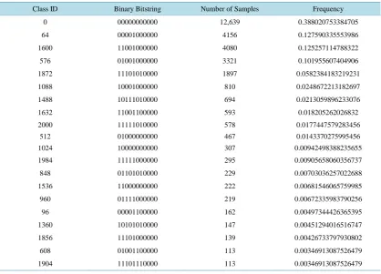
From our collection of boolean profiles, we determined the number of samples that were in each class. Figure 1 shows the number of samples in each class. Many of the classes show almost no members; there were 116 classes that did. A list of the top 20 is shown in Table 1.
Figure 1. Frequency of class membership (x = class bitstring number).
Table 1. Top 20 Malware classes in our corpus as defined by our bitstring scheme, ordered by class membership.
Class ID Binary Bitstring Number of Samples Frequency
0 00000000000 12,639 0.388020753384705
64 00001000000 4156 0.127590335553986
1600 11001000000 4080 0.125257114788322
576 01001000000 3321 0.101955607404906
1872 11101010000 1897 0.0582384183219231
1088 10001000000 810 0.0248672213182697
1488 10111010000 694 0.0213059896233076
1632 11001100000 593 0.018205262026832
2000 11111010000 578 0.0177447579283456
512 01000000000 467 0.0143370275995456
1024 10000000000 307 0.00942498388235655
1984 11111000000 295 0.00905658060356737
848 01101010000 229 0.00703036257022688
1536 11000000000 222 0.00681546065759985
960 01111000000 219 0.00672335983790256
96 00001100000 162 0.00497344426365395
1360 10101010000 147 0.00451294016516747
1856 11101000000 139 0.00426733797930802
608 01001100000 113 0.00346913087526479
[image:5.595.89.508.425.726.2]Class 0 used was closed; the Sandbox therefore represented a more modern iteration of the operating system in which some of the security problems were fixed.
By ranking the frequencies of each class, we see that the frequencies drop dramatically after the first class, after which the decrease in frequency is much less dramatic. Figure 2 shows the frequency distribution on a log scale. We see that certain classes of malware are rarer in the wild than others, although the reason for this is dif-ficult to know. Possibilities include program complexity and the ease in which a sample within a particular class can infect computers, both of which are the subject of future research.
Examining the frequency rankings, we found that the frequencies tended to follow a power-law distribution. Our data shows that our corpus approximately follows an expected power law curve.
Class 64 (00001000000) Class 64 malware samples exhibit only Process creation. Nevertheless, we see many types of malware within this class, such as worms, download Trojans, spyware Trojans, and even some that tar-get Linux instead of Windows. In these cases, it would appear that the process created in memory is what per-formed many of the tasks, often beyond the reach of the analysis tool.
Class 1600 (11001000000) Class 1600 malware exhibits File System, Registry and Process creation proper-ties. These samples may read and write files on the computer, enumerate and alter registry settings, and create processes in memory. The changes to the file system or registry may be performed by the main program, or by a spawned process. Note that Registry operations do not necessarily imply file system changes; Norman Sandbox differentiates between the two kinds of activity.
Class 576 (01001000000) Class 576 malware exhibits Registry and Process creation properties. There are many ways that this could be leveraged as the registry is capable of storing information and code, which could be run at a later time. One way that this could happen is if the malware sample creates a process that runs, using information from the registry to act. Alternatively, the process could also be operating directly on the registry, instead of using it as a “seed” for code.
[image:6.595.103.502.417.705.2]Class 1872 (11101010000) Class 1872 malware exhibits File System, Registry, Network, Process creation and Network service properties. Network and Network Services tend to go hand-in-hand-network refers to the use of network traffic by a malware sample, whereas network services refers to higher level network operations,
such as connecting to an IRC server or starting a web server. A sample in this class, for example, might alter the registry to allow for a program to start on boot (to ensure that its programs are always running), then connect over a network to download an executable program, which is then written to disk and run. The spawned process will then perform whatever acts it wishes, and due to the registry change, will start up on boot to continue to act upon the system.
Class 1088 (10001000000) Class 1088 malware exhibits File system and Process creation properties. Mem-bers of this class could write small programs to act on the system to disk, and then subsequently execute those programs.
4.1. Complexity over Time
We hypothesize that malware complexity will increase over time, both because of and in order to take advantage of the increasing complex nature of computer systems. Our hypothesis is that a more complicated piece of mal-ware (defined as a sample that exhibits more properties than a less complex sample) will appear after simpler malware, chronologically. We do not deny the fact that a “simple” type of malware may continue to exist and infect; it is possible that some of those samples are uniquely fit to survive the changing computer landscape.
We examined malware samples in pairs from our dated corpus, using the algorithm defined in Algorithm 4.1. First, we defined two functions-ones X
( )
which returns the string of positive boolean values in sample X s′profile, including position within the string, and date X
( )
, which returns the discovery date of sample Xthrough a lookup.
Algorithm 1 Algorithm to compare a set of samples in terms of bitstring complexity. {M isourdatedmalwarecorpus}
for all P Q, ∈M do If P = Qthen
next;{Wedonotcompareasampletoitself} end if
if ones
( )
P ⊂ones( )
Q then totalcompares←totalcompares 1+ if date( )
P < date( )
Q thenpositivecompares←positivecompares 1+ else
negativecompares←negativecompares 1+ end if
end if end for
(
)
ratio←positivecompares positivecompares+negativecompares
By comparing all pairs in M, there were over 1,000,000,000 possible pairwise comparisons. Of these compar-isons, 379,950,237 pairs were checked where one sample’s properties were a subset of the other. 52.4%, or 199,113,920 comparisons supported our theory, while 180,836,317 rejected it. This result was skewed due to the differing numbers of samples within each class. This algorithm looks at any arbitrary pair of samples, so there were pairs that would be compared twice, one time which would support our hypothesis and one which would not. We then refined our measure by first filtering out samples so that we were able to determine the “progenitor” of each malware class-the sample at which a particular bitstring first appeared. This was accomplished by ex-amining the corpus, and, for each sample, checking if its discovery date was the earliest for its respective class. If it was, we kept it as a “progenitor” of that class. At the end, we had a total of 116 samples left to check. We then ran the corpus through the same algorithm and found that, of the 13,340 possible pairwise comparisons, there were 1580 comparisons where one sample was a subset of the other. Of those, 82.7%, or 1306 supported our hypothesis and 274 rejected it.
4.2. Longevity of Malware Classes
class, and find out how long that class persists in our corpus. By examining the samples in the corpus and de-termining, for each class, the date of the first appearance and the date of the last one, we were able to determine the longevity of each class within our corpus. The average longevity for a malware class was approximately 1648 days, ranging from 0 days to 6438 days. A longevity of 0 days indicates that the first and last appearance of a class was on the same day, which could indicate that a particular class was ineffective at spreading, or that that particular class did not spawn many variants within the same class. It does not exclude the possibility that the class served as the basis for a more complex class, however. A higher longevity number does indicate that the class is uniquely suited for survival-while the specific exploits that different samples within the class employ may differ, the overall behavior remains constant and therefore that kind of attack that a sample in that class represents remains possible for a longer amount of time.
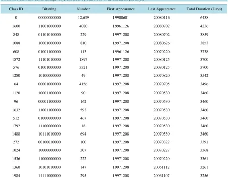
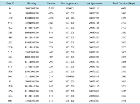
Table 2 and Table 3 show the longevity of the various classes, ordered by the length of time that a class was active, and the number of samples within that class, respectively. We see that for the most part, there is a corre-lation between the number of samples and the length of time that a malware class is active-the more samples of a class that exist, the longer that class is able to survive. This can be attributed to the fact that even if a sample is particularly virulent and has a profound effect on a computer, if new samples that are similar to it are not created, eventually anti-virus and anti-malware programs will be able to eradicate that sample and other members of its class. Without new samples being created within a class, said class will eventually die out in favor of newer, possibly more complex ones, that take advantage of more of the features available to a malware writer.
5. Conclusions and Further Work
Our method creates malware classification that creates a simple, human-readable classification system. The ad-
Table 2. Malware Class Longevity, ordered by class survival duration (in days).
Class ID Bitstring Number First Appearance Last Appearance Total Duration (Days)
0 00000000000 12,639 19900601 20080116 6438
1600 11001000000 4080 19961126 20080702 4236
848 01101010000 229 19971208 20080702 3859
1088 10001000000 810 19971208 20080626 3853
608 01001100000 113 19961126 20070220 3738
1872 11101010000 1897 19971208 20080125 3700
576 01001000000 3321 19971208 20080125 3700
1280 10100000000 49 19971208 20070820 3542
64 00001000000 4156 19971208 20070705 3496
1120 10001100000 90 19971208 20070530 3460
96 00001100000 162 19971208 20070530 3460
1632 11001100000 593 19971208 20070530 3460
512 01000000000 467 19971208 20070530 3460
1792 11100000000 18 19971208 20070530 3460
1488 10111010000 694 19971208 20070530 3460
272 00100010000 100 19971208 20070322 3391
1024 10000000000 307 19971208 20070227 3368
1536 11000000000 222 19971208 20070220 3361
1360 10101010000 147 19971208 20061112 3261
Table 3. Malware Class Longevity, ordered by class membership.
Class ID Bitstring Number First Appearance Last Appearance Total Duration (Days)
0 00000000000 12,639 19900601 20080116 6438
64 00001000000 4156 19971208 20070705 3496
1600 11001000000 4080 19961126 20080702 4236
576 01001000000 3321 19971208 20080125 3700
1872 11101010000 1897 19971208 20080125 3700
1088 10001000000 810 19971208 20080626 3853
1488 10111010000 694 19971208 20070530 3460
1632 11001100000 593 19971208 20070530 3460
2000 11111010000 578 19971208 20060915 3203
512 01000000000 467 19971208 20070530 3460
1024 10000000000 307 19971208 20070227 3368
1984 11111000000 295 19971208 20061107 3256
848 01101010000 229 19971208 20080702 3859
1536 11000000000 222 19971208 20070220 3361
960 01111000000 219 19980616 20060814 2981
96 00001100000 162 19971208 20070530 3460
1360 10101010000 147 19971208 20061112 3261
1856 11101000000 139 19971208 20060818 3175
1904 11101110000 113 19971208 20060817 3174
608 01001100000 113 19961126 20070220 3738
vantage of this system is that, due to the limited number of possible classes, it is possible to create a look-up ta-ble of malware behavior; a new sample that is examined and exhibits behavior can immediately be grouped with samples that have similar behavior. At that point, further, more directed analysis can be done. The disadvantage of this method is the overhead involved with the classification; while determining boolean class is quick, since we are performing dynamic analysis, we are bound by the time it takes to perform an execution of the sample. Of course, this means that this method is also subject to some of the pitfalls of dynamic analysis; some samples are able to detect that they are being used within a sandboxed environment and can adjust their execution accor-dingly [2].
Going forwards, this method is most useful as a sort of pre-processing phase of a collection of malware; when comparing samples to each other we have found that often it is wasteful to compare samples that are unrelated to each other; that the relationship between malware samples when grouping them into families is facilitated when samples that are more closely related are set to be grouped together.
Finally, this method can be used to classify very specific behavior, given that classification of behaviors can be as fine-grained as desired. A detector can be programmed to look for any operation within a category of be-havior; if we are looking at registry changes, we can design our scheme to look for the most specific registry change we want to use as a basis of classification. This level of customization allows for more targeted detectors which, while not always useful in the real-world, are useful in an isolated setting as part of a reverse-engineering approach.
References
[1] Classification of Species, 2009.
https://web.archive.org/web/20120121022919/http://classes.entom.wsu.edu/348/classification.htm
[2] Seideman, J. (2009) Recent Advances in Malware Detection and Classification: A Survey. Technical Report, The Graduate School and University Center of the City University of New York.
[3] Spafford, E.H. (1994) Computer Viruses as Artificial Life. Artificial Life, 1, 249-265.
http://dx.doi.org/10.1162/artl.1994.1.3.249
[4] Bailey, M., Oberheide, J., Andersen, J., Morley Mao, Z.Q., Jahanian, F. and Nazario, J. (2007) Automated Classifica-tion and Analysis of Internet Malware. Proceedings of RAID 2007, 178-197.
http://dx.doi.org/10.1007/978-3-540-74320-0_10.
[5] Riau, C. (2002) A Virus by Any Other Name: Virus Naming Practices.
http://www.symantec.com/connect/articles/virus-any-other-name-virus-naming-practices
[6] Gandotra, E., Bansal, D. and Sofat, S. (2014) Malware Analysis and Classification: A Survey. Journal of Information Security, 5, 56-64.http://dx.doi.org/10.4236/jis.2014.52006
[7] Lee, T. and Mody, J.J. (2006) Behavioral Classification. Proceedings of EICAR 2006, May 2006, 1-17. [8] Szor, P. (2005) The Art of Computer Virus Research and Defense. Addison-Wesley, New York.
[9] Jacob, G., Debar, H. and Filiol, E. (2008) Behavioral Detection of Malware: From a Survey towards an Established Taxonomy. Journal in Computer Virology, 4, 251-266.http://dx.doi.org/10.1007/s11416-008-0086-0
[10] Andreas Moser, Christopher Kr¨ugel, and Engin Kirda. (2007) Exploring Multiple Execution Paths for Malware Anal-ysis. Proceedings of the 2007 IEEE Symposium on Security and Privacy, 2007, 231-245.
http://dx.doi.org/10.1109/SP.2007.17
[11] (2009) Norman Sandbox.
https://web.archive.org/web/20101005091013/http://www.norman.com/technology/norman_sandbox/
[12] Liang, Z.K., Sun, W.Q., Venkatakrishnan, V.N. and Sekar, R. (2009) Alcatraz: An Isolated Environment for Experi-menting with Untrusted Software. ACM Transactions on Information and System Security, 12, 1-37.
[13] Buyrukbilen, S. and Deryol, R. (2008) An Automated System for Behavioral Malware Analyis. Technical Report, John Jay College of Criminal Justice, City University of New York.
[14] (2010) The Honeynet Project. http://www.honeynet.org
[15] (2010) Nepenthes—Finest Collection. http://nepenthes.carnivore.it/
[16] (2012) Dionaea-Catches Bugs. http://dionaea.carnivore.it/
[17] (2010) Offensive Computing: Community Malicious Code Research and Analysis.
http://www.offensivecomputing.net [18] VX Heavens, 2010. http://vxheaven.org/
[19] Symantec, 2012. http://www.symantec.com/index.jsp
[20] VirusTotal, 2008. http://www.virustotal.com
[21] (2012) Threat Explorer—Spyware and Adware, Dialers, Hack Tools, Hoaxes and Other Risks.
http://www.symantec.com/security_response/threatexplorer/