A Kind of Doubly Periodic Riemann Boundary Value Problem on Two Parallel Curves

(1)

http://dx.doi.org/10.4236/apm.2014.412071

A Kind of Doubly Periodic Riemann

Boundary Value Problem on Two Parallel

Curves

Lixia Cao, Xiaowei Li, Chengxin Lin

School of Mathematics and Statistics, Northeast Petroleum University, Daqing, China Email: [email protected]

Received 6 November 2014; revised 3 December 2014; accepted 9 December 2014

This work is licensed under the Creative Commons Attribution International License (CC BY). http://creativecommons.org/licenses/by/4.0/

Abstract

We proposed a kind of doubly periodic Riemann boundary value problem on two parallel curves. By using the method of complex functions, we investigated the method for solving this kind of dou- bly periodic Riemann boundary value problem of normal type and gave the general solutions and the solvable conditions for it.

Keywords

Normal Type, Doubly Periodic, Riemann Boundary Problem

1. Introduction

Various kinds of Riemann boundary value problems (BVPs) for analytic functions on closed curves or on open arcs, doubly periodic Riemann BVPs, doubly periodic or quasi-periodic Riemann BVPs and Dirichlet Problems, and BVPs for polyanalytic functions have been widely investigated in papers [1]-[8]. The main approach is to use the decomposition of polyanalytic functions and their generalization to transform the boundary value prob-lems to their corresponding boundary value probprob-lems for analytic functions. Recently, inverse Riemann BVPs for generalized analytic functions or bianalytic functions have been investigated in papers [9]-[13].

In this paper, we consider a kind of doubly periodic Riemann boundary value problem on two parallel curves. By using the method of complex functions, we investigate the method for solving kind of doubly periodic Rie-mann boundary value problem of normal type and give the general solutions and the solvable conditions for it.

2. A Kind of Doubly Periodic Riemann Boundary Value Problem on Two Parallel

Curves

(2)

pa-rallelogram with vertices ± ±ω ω₁ ₂. The function

( )

(

)

2

,

1 ' 1 mn 1 mn mn

m n

z z z z

ζ = +

∑

_ − Ω + Ω + Ω _

is called the Weierstrass ζ -function, where Ω =mn 2mω1+2nω2, and ,

' m n

∑

denotes the sum for all m, 0, 1, 2,

n= ± ± , except for m= =n 0. Let

2

0 0

1

j j

L L

=

∑

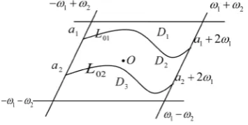
be the set of two parallel curves, lying entirely in the fundamental period parallelogram P, not passing the origin O, with endpoints being periodic congruent and having the same tangent lines at the pe-riodic congruent points. Let D₁, D₂, D₃ denote the domains entirely in the fundamental period parallelogram

P, cut by L₀₁ and L₀₂, respectively. Without loss of generality, we suppose that O∈D₂, see Figure 1. Let

01

L∗ , L∗₀₂ be the curves periodically extended for L₀₁ and L₀₂ with period 2ω₁, respectively. And L∗_nj

(

j=1, 2;n= ±0, 1,

)

be the curves periodically extended for L0j

∗

with 2nω₂.

Our objective is to find sectionally holomorphic doubly periodic functions F z

( )

and Ω

( )

z , satisfying the following boundary conditions

( )

( ) ( )

( )

( ) ( )

( )

1 1 01

2 2 02

, , , ,

F D g L

D F g L

τ τ τ τ τ τ τ τ τ τ

+ −

 = Ω + ∈

 

Ω = + ∈

 (1)

where Dj

( )

τ , gj

( )

τ ∈H, and be doubly periodic with 2ω1, 2ω2. F

( )

τ ±

are the boundary values of the function F z

( )

, which is analytic in D1 and D3, belonging to the class h a

( )

j on L0j, satisfying the boun-

dary conditions (1), and Ω±

( )

τ

are the boundary values of the function Ω

( )

z , which is analytic in D2,

be-longing to the class h a

( )

_j on L₀_j, satisfying the boundary conditions (1).

Since aj plays the same roles as other points on L0j

(

j=1, 2

)

, it is natural to require that the unknown

functions are bounded at z=a_j, that is, the unknown functions F z

( )

and Ω

( )

z are both bounded on L∗₀₁

and L∗₀₂.

Problem (1) is called the normal type if D_j

( )

τ ≠0

(

j=1, 2

)

, otherwise the non-normal type. And if we allow the solution Ω

( )

z has poles of order m at z = 0, it is actually to solve problem (1) in DR_m.

3. Preliminary Notes

Since D_j

( )

τ ∈H with D_j

( )

τ ≠0

(

j=1, 2

)

, by taking logarithm of logD_j

( )

τ for some branch on L₀_j, we may obtain a continuous single-valued function such as

( )

(

)

1

log , 1, 2,

2π 1

log 2 , 1, 2.

2π

j j

j j a a

j j j a a

D a i j

i

D a i j

i

α β

ω α β

− = + =

+ = − − =

with 0 1

j

a

α

≤ < . Now we call the integer κ κ κ= 1+ 2 the index of problem (1), where κj is the integer

[image:2.595.226.404.606.696.2]

sa-tisfying

(3)

0≤ −αa_j −κj <1, j=1, 2.

Since κj can only be 0 and −1, the index

κ

can only take 0, 1, 2− − .

Set

( )

01 02

1 2 1 2

1 1

log log d

2π L 2π L

D D D D D

i

τ

i

τ τ

∗ = ∗+ ∗ =

∫

+

∫

(2)

( )

( ) (

)

0 0

1

log d , , 1, 2 2π j

j z _L Dj z z L j j

i

γ

=

_∫

τ ξ τ

−

τ

∉ = (3)

We can easily see that 1 eγj( )z _{will have singularities at most less than one order near the endpoints}

j

a and

1 2 j

a + ω

(

j=1, 2

)

. Let

( ) 1( ) 2( )

eγ z =eγ zeγ z (4) then we have

( 2 ) 2 ( )

eγ z+ ωj ₌e−ηjD∗eγ z _, j=1, 2_,

where

η

j =

ζ ω

( )

j

(

j=1, 2

)

and 2ω η2 1−2ω η1 2=πi. Thus ( )

eγ z is not doubly periodic generally. In fact,

( )

eγ z is doubly periodic if and only if

π jD kj i

η _∗= , k_j is positive integer for j=1, 2. (5)

Lemma 1. Formula (5) is valid if and only if

1 2 k k1 2

η η = , D∗=2k1ω2−2k2ω1.

And if both D∗=2l1ω1+2l2ω2 and ηjD∗=kjπi are true, then we have l1= −k2 and l2=k1, where lj, j

k are all integers.

4. Solution for Problem (1) of Normal Type

Problem (1) can be transferred by using (3) as

( )

1 1 1

2 2 2

1

01

2

02 , ,

e e e

.

e e e

F g

L

F g

L

γ τ γ τ γ τ

τ τ τ τ τ τ τ

τ

+ − +

+ −

 Ω

= + ∈

  

Ω

 ₌ ₊ _∈

 

(6)

Multiplying _{( )}

2

1 eγ τ−

to the two sides of the first identity in equations (6), and multiplying _{( )}

1

1 eγ τ−

to the two sides of the second identity in Equations (6), gives

( )

( ) ( )

( )

( ) ( )

( )

( ) ( )

( )

( ) ( )

( )

( ) ( )

( )

( ) ( )

1 2 1 2 1 2

2 1 2 1 2 1

1

01

2

02 , ,

e e e e e e

.

e e e e e e

F g

L

F g

L

γ τ γ τ γ τ γ τ γ τ γ τ

τ τ τ

τ

τ τ τ

τ

+ − − − + −

+ −

 Ω

= + ∈

  

Ω

 ₌ ₊ _∈

 

(7)

The function 1 eγj( )z _{always has singularities at most less than one order near the endpoints}

j

a and

1 2 j

a + ω

(

j=1, 2

)

whatever

κ

= − −0, 1, 2. And then, _{( )}

( )

_{( )}

1 2

1

e e

g

γ τ γ τ

τ

+ − ,

( )

( ) ( )

2 1

2

e e

g

γ τ γ τ

τ

+ − must belong to class H or class H*_on_L

01 and L02, respectively.

Case 1. If formula (5) holds, that is, eγ( )z is doubly periodic, then by Lemma 1 we have

(

1 2

)

0 mod 2 , 2

(4)

( )

_{( )}

( )

_{( )}

(

)

( )

01 1 2

1

1 01

1

d , 2π L _e _e

g

z z z z L

i γ τ γ τ

τ

ζ τ ζ τ

+ −

Ψ =

_∫

_ − + _ ∉ (9)

( )

_{( )}

( )

_{( )}

(

)

( )

02 2 1

2

2 02

1

d , 2π L _e _e

g

z z z z L

i γ τ γ τ

τ

ζ τ ζ τ

+ −

Ψ =

_∫

_ − + _ ∉ (10)

Then by formulas (9) and (10), we may rewrite (7) as

( )

( ) ( )

( )

( ) ( )

( )

( ) ( )

( )

( ) ( )

( )

1 2 1 2

2 1 2 1

1 2 1 2 01

1 2 1 2 02

,

e e e e

,

e e e e

F

L

F

L

γ τ γ τ γ τ γ τ

τ τ

τ τ τ τ τ

τ τ

τ τ τ τ τ

+ − − − + − − − + − + + − + + − − + − −  Ω

− Ψ − Ψ = − Ψ − Ψ ∈ 

 

Ω

 _{− Ψ} _{− Ψ} ₌ _{− Ψ} _{− Ψ} _∈ 



(11)

Now we introduce the function

( )

1 2 1

1 1 2 2

1 2 3

, , e , , e , , e z z z F z

z z z D

z

z z z z D

F z

z z z D

γ γ γ + + + − − + − − − 

− Ψ − Ψ ∈

  Ω 

Φ = − Ψ − Ψ ∈

 

 − Ψ − Ψ ∈



then Φ1

( )

z has n-order at z = 0, and has singularities at most less than one order near the endpoints aj and

1 2 j

a + ω

(

j=1, 2

)

. Thus we can get the following results.

1° When m > 0, problem (1) is solvable without any restrictive conditions and the general solution is given by

( )

_{( )}

( )

_{( )}

( )

_{( )}

1

0 1 1 1 2 1

1

0 1 1 1 2 2

1

0 1 1 1 2 3

e , ,

z m m z m m z m m

F z c c z c z z z z D

z c c z c z z z z D

F z c c z c z z z z D

γ γ γ ζ ζ ζ ζ ζ ζ + − + + − − − + − − − − − −

 = _ + ′ + + + Ψ + Ψ _ ∈ 

_Ω ₌ _ ₊ _′ _{+ +} _{+ Ψ} _{+ Ψ} _ _∈

 _ _



 ′ 

= + + + + Ψ + Ψ ∈

 _ _     (12)

where c c0, ,1,cm−1 are arbitrary constants.

2° When m = 0, problem (1) is solvable if and only if the restrictive conditions

( )

( ) ( )

( )

( ) ( )

01 1 2

02 2 1

1

2 1

d 0,

2π _e _e

1

d 0,

2π _e _e

L L g i g i

γ τ γ τ

τ τ τ τ + − + −  =     ₌ 

∫

(13)

are satisfied, and now the solution is given by

( )

_{( )}

( )

_{( )}

( )

_{( )}

1 2 1

1 2 2

1 2 3

e , ,

z

F z c z z z D

z c z z z D

F z c z z z D

γ γ γ + + + − + − − −

 = _ + Ψ + Ψ _ ∈ 

_Ω ₌ _ _{+ Ψ} _{+ Ψ} _ _∈

 _ _



 

= + Ψ + Ψ ∈

 _ _



(14)

where c is arbitrary constant.

3° When m < 0, if and only if the restrictive conditions (13) and

( )

( ) ( )

( )

( ) ( )

( )

01 1 2

02 2 1

1

2 1

d 0

2π _e _e

1, 2, , 1, 1

d 0

2π _e _e

k L k L g i k m g i

γ τ γ τ

τ

ζ τ τ τ

ζ τ τ

+ − + −  =   ₌ _{− −}   ₌ 

∫

(5)

(when m= −1, the condition (15) is unnecessary) are necessary, problem (1) is solvable and the solution can still be given by (14) but with

( ) ( )

01 1 2 02 2 1

1 2

1 1

d d

2π _e _e 2π _e _e

k k

L L

g g

c

i γ τ γ τ i γ τ γ τ

τ ζ τ τ ζ τ

τ τ

+ − + −

= −

_∫

−

_∫

,

Case 2. If formula (5) fails to hold, then by Lemma 1 we see that D∗≠0. Let

( )

( ) (

)

h_∗ z =σ z σ z−D_∗ ,

then the function eγ( )zh z_∗

( )

become doubly periodic, and function _{( )}

( )

1

eγzh z_∗ has singularities at most less

than one order near the endpoints aj and aj+2ω1

(

j=1, 2

)

. Thus now, we can transform (6) to

( )

( ) ( )

_{( )}

( )

( ) ( )

_{( )}

( )

( ) ( )

_{( )}

( )

( ) ( )

_{( )}

( )

( ) ( )

_{( )}

( )

( ) ( )

_{( )}

1 2 1 2 1 2

2 1 2 1 2 1

1 01 * 2 02 , ,

e e e e e e

, .

e e e e e e

F g

L

h h h

F g

L

h h h

γ τ γ τ γ τ γ τ γ τ γ τ

τ τ τ

τ

τ τ τ

τ

τ τ τ

+ − − − + − + − − − − − + − ∗ ∗ + − ∗ ∗ ∗  Ω = + ∈    Ω  ₌ ₊ _∈   (16)

where _{( )}

( )

_{( )}

( )

1 2 1 e e g h γ τ γ τ

τ τ + − ∗ , _{( )}

( )

_{( )}

( )

2 1 2 e e g h γ τ γ τ

τ τ

+ −

∗

belong to class H or class H*_on_L

01 and L02, respectively. Write

( )

_{( )}

( )

_{( )}

( )

(

)

( )

01 1 2

1

1 01

1

d , 2π L _e _e

g

z z z z L

i γ τ γ τ _h

τ

ζ τ ζ τ τ

+ −

∗

Ψ =

_∫

_ − + _ ∉ ₍₁₇₎

( )

_{( )}

( )

_{( )}

( )

(

)

( )

02 2 1

2

2 02

1

d , 2π L _e _e

g

z z z z L

i γ τ γ τ _h

τ

ζ τ ζ τ τ

+ −

∗

Ψ =

_∫

_ − + _ ∉ ₍₁₈₎

By (17) and (18), we can rewrite (16) as

( )

( ) ( )

_{( )}

( )

( ) ( )

_{( )}

( )

( ) ( )

_{( )}

( )

( ) ( )

_{( )}

( )

1 2 1 2

2 1 2 1

1 2 1 2 01

1 2 1 2 02

, ,

e e e e

, .

e e e e

F L h h F L h h

γ τ γ τ γ τ γ τ

τ τ

τ τ τ τ τ

τ τ

τ τ τ τ τ

τ τ + − − − + − − − + − + + − + ∗ ∗ ∗ ∗ ∗ ∗ + − − + − − ∗ ∗ ∗ ∗ ∗ ∗  Ω

− Ψ − Ψ = − Ψ − Ψ ∈ 

 

Ω

 _{− Ψ} _{− Ψ} ₌ _{− Ψ} _{− Ψ} _∈ 



(19)

Now we will meet two kinds of situations in solving problem (1) in DR_m.

(a) When D∗ ≡0 mod 2

(

ω ω1, 2 2

)

, the function h z∗

( )

is an entire function. And we can write it without

counting nonzero constant as

( )

exp 2

{

(

1 1 2 2

)

}

h z∗ = l

η

+l

η

,

where l₁, l₂ are determined by the identity D∗=2l₁ω₁+2l₂ω₂.

1° When m > 0, problem (1) is solvable without any restrictive conditions and the general solution is given by

( )

_{( )}

( )

_{( )}

( )

_{( )}

1

0 1 1 1 2 1

1

0 1 1 1 2 2

1

0 1 1 1 2 3

e , ,

z m m z m m z m m

F z h z c c z c z z z z D

z h z c c z c z z z z D

γ γ γ ζ ζ ζ ζ ζ ζ + − + + ∗ − ∗ ∗ − − − ∗ − ∗ ∗ − − − − ∗ − ∗ ∗

 = _ + ′ + + + Ψ + Ψ _ ∈ 

_Ω ₌ _ ₊ _′ _{+ +} _{+ Ψ} _{+ Ψ} _ _∈

 _ _



 ′ 

= + + + + Ψ + Ψ ∈

 _ _     (20)

where c c0, ,1,cm−1 are arbitrary constants.

(6)

( )

( ) ( )

_{( )}

( )

( ) ( )

_{( )}

01 1 2

02 2 1

1

2

1

d 0,

2π _e _e

1

d 0,

2π _e _e

L L g i _h g i _h

γ τ γ τ

τ τ τ τ τ τ + − + − ∗ ∗  =     ₌  

∫

(21)

are satisfied, and the general solution for (1) is given by

( )

_{( )}

( )

_{( )}

( )

_{( )}

1 2 1

1 2 2

1 2 3

e , ,

z

F z h z c z z z D

z h z c z z z D

F z h z c z z z D

γ γ γ + + + ∗ ∗ ∗ − + ∗ ∗ ∗ − − − ∗ ∗ ∗

 = _ + Ψ + Ψ _ ∈ 

_Ω ₌ _ _{+ Ψ} _{+ Ψ} _ _∈

 _ _



 

= + Ψ + Ψ ∈

 _ _



(22)

where c is arbitrary constant.

3° When m < 0, if and only if the restrictive conditions (21) and

( )

( ) ( )

_{( )}

( )

_{( )}

( )

( ) ( )

_{( )}

( )

_{( )}

1 2 02

02 2 1

1

2

1

d 0,

2π _e _e

1, 2, , 1. 1

d 0,

2π _e _e

k L k L g i _h k m g i _h

γ τ γ τ

τ

ζ τ τ τ

τ

ζ τ τ τ + − + − ∗ ∗  =   = −   ₌  

∫

 (23)

(when m= −1, the condition (23) is unnecessary) are both necessary, problem (1) is solvable and the solution can still be given by (22) but with

( )

( ) ( )

_{( )}

( )

( ) ( )

_{( )}

01 1 2 02 2 1

1 2

1 1

d d

2π L _e _e 2π L _e _e

g g

c

i γ τ γ τ_h i γ τ γ τ_h

τ τ τ τ τ τ + − + − ∗ ∗ = −

_∫

−

_∫

_.

(b) When D∗ ≡0 mod 2

(

ω ω1, 2 2

)

fails to hold, the function ( )

( )

1

eγzh z_∗ has singularity of one order at z = 0,

has singularities at most less than one order near the endpoints aj and aj+2ω1

(

j=1, 2

)

, and has a zero of

order one at z=D∗. Write

( )

_{( )}

( )

_{( )}

( )

_{( )}

( )

1 2 1

1 1 2 2

1 2 3

, , e , , e , , e z z z F z

z z z D

h z

z

z z z z D

h z

F z

z z z D

h z γ γ γ + + + ∗ ∗ ∗ − + ∗ ∗ ∗ − − − ∗ ∗ ∗ 

 − Ψ − Ψ ∈

 

Ω 

Φ =_ − Ψ − Ψ ∈

 

 _{− Ψ} _{− Ψ} _∈

 

(24)

then Φ₁

( )

z must be at most m + 1 ordered at z = 0, and has singularities less than one order at z = aj (j = 1, 2).

1° When m≥0, problem (1) is solvable without any restrictive conditions and the general solution is given by

( )

_{( )}

( )

_{( )}

( )

_{( )}

0 1 1 2 1

0 1 1 2 2

0 1 1 2 3

e , ,

z m m z m m z m m

z h z c c z c z z z z D

γ γ γ ζ ζ ζ ζ ζ ζ + + + ∗ ∗ ∗ − + ∗ ∗ ∗ − − − ∗ ∗ ∗

 = _ + ′ + + + Ψ + Ψ _ ∈ 

_Ω ₌ _ ₊ _′ _{+ +} _{+ Ψ} _{+ Ψ} _ _∈

 _ _



 ′ 

= + + + + Ψ + Ψ ∈

 _ _     (25)

with the restrictive condition that

( )

_{( )}

0 1 1 2 0

m m

c = −c

ζ

′ D∗ − − c

ζ

D∗ − Ψ∗ D∗ − Ψ∗ D∗ = ,

(7)

( )

_{( )}

0 1 1 1 2

m m

c = −c

ζ

′ D∗ − − c −

ζ

D∗ − Ψ∗ D∗ − Ψ∗ D∗ ,

where c c1, 2,,cm are arbitrary constants, which is to ensure that Φ1

( )

D∗ =0, that is, to ensure F

( )

D

± ∗

and Ω

( )

D_∗ be bounded.

2° When m= −1, problem (1) is solvable if and only if the restrictive conditions

( )

( ) ( )

_{( )}

( )

( ) ( )

_{( )}

01 1 2

02 2 1

1

2

1

d 0,

2π _e _e

1

d 0,

2π _e _e

L L g i _h g i _h

γ τ γ τ

τ τ τ τ τ τ + − + − ∗ ∗  =     ₌  

∫

(26)

are satisfied, and now the solution is given by

( )

_{( )}

( )

_{( )}

( )

_{( )}

1 2 1 2 1

1 2 1 2 2

1 2 1 2 3

e , ,

z

F z h z z z D D z D

z h z z z D D z D

F z h z z z D D z D

γ γ γ + + + ∗ ∗ ∗ ∗ ∗ ∗ ∗ − + ∗ ∗ ∗ ∗ ∗ ∗ ∗ − − − ∗ ∗ ∗ ∗ ∗ ∗ ∗

 = _Ψ + Ψ − Ψ − Ψ _ ∈ 

_Ω ₌ __Ψ _{+ Ψ} _{− Ψ} _{− Ψ} _ _∈

 _ _



 

= Ψ + Ψ − Ψ − Ψ ∈

 _ _



(27)

which is finite at z=D∗ owing to its structure.

3° When m< −1, problem (1) is solvable if and only if both conditions (26) and the following conditions

( ) ( )

(

)

( ) ( )

_{( )}

( ) ( )

(

)

( ) ( )

_{( )}

01 1 2

02 2 1

1

2 1

d 0,

2π _e _e

1

d 0,

2π _e _e

L L g D i _h g D i _h

γ τ γ τ

τ ζ τ ζ τ

τ τ

τ ζ τ ζ τ

τ τ + − + − ∗ ∗ ∗ ∗  _ − − _ =    − −      ₌  

∫

(28)

( )

( ) ( )

_{( )}

( )

_{( )}

( )

( ) ( )

_{( )}

( )

_{( )}

01 1 2

02 2 1

1

2

1

d 0,

2π _e _e

1, 2, , 1 1

d 0,

2π _e _e

k L k L g i _h k m g i _h

γ τ γ τ

τ

ζ τ τ τ

τ

ζ τ τ τ + − + − ∗ ∗  =   = − −   ₌  

∫

 (29)

(when m= −2, (28) is unnecessary) are necessary, and the solution is given by

( )

_{( )}

( )

_{( )}

( )

_{( )}

1 2 1 2 1

1 2 1 2 2

1 2 1 2 3

e 0 0 , ,

e 0 0 , .

z

F z h z z z z D

z h z z z z D

F z h z z z z D

γ γ γ + + + ∗ ∗ ∗ ∗ ∗ − + ∗ ∗ ∗ ∗ ∗ − − − ∗ ∗ ∗ ∗ ∗

 = _Ψ + Ψ − Ψ − Ψ _ ∈ 

_Ω ₌ __Ψ _{+ Ψ} _{− Ψ} _{− Ψ} _ _∈

 _ _



 

= Ψ + Ψ − Ψ − Ψ ∈

 _ _



(30)

which is finite at z=D∗ owing to its structure.

Funding

The project of this thesis is supported by “Heilongjiang Province Education Department Natural Science Re-search Item”, China (12541089).

References

[1] Balk, M.B. (1991) Polyanalytic Functions. Akademie Verlag, Berlin.

[2] Begehr, H. and Kumar, A. (2005) Boundary Value Problems for the Inhomogeneous Polyanalytic Equation I. Analysis:

International Mathematical Journal of Analysis and its Application, 25, 55-71.

[3] Du, J.Y. and Wang, Y.F. (2003) On Boundary Value Problems of Polyanalytic Functions on the Real Axis. Complex

(8)

[4] Fatulaev, B.F. (2001) The Main Haseman Type Boundary Value Problem for Metaanalytic Function in the Case of Circular Domains. Mathematical Modelling and Analysis, 6, 68-76.

[5] Lu, J.K. (1993) Boundary Value Problems for Analytic Functions. World Scientific, Singapore.

[6] Mshimba, A.S. (2002) A Mixed Boundary Value Problem for Polyanalytic Function of Order n in the Sobolev Space

Wn, p(D). Complex Variables, 47, 278-1077.

[7] Muskhelishvili, N.I. (1993) Singular Integral Equations. World Scientific, Singapore.

[8] Wanf, Y.F. and Du, J.Y. (2006) Hilbert Boundary Value Problems of Polyanalytic Functions on the Unit Circumfe-rence. Complex Variables and Elliptic Equations, 51, 923-943. http://dx.doi.org/10.1080/17476930600667692

[9] Xing, L. (1995) A Class of Periodic Riemann Boundary Value Inverse Problems. Proceedings of the Second Asian

Mathematical Conference, Nakhon Ratchasima, October 1995, 397-400.

[10] Wang, M.H. (2006) Inverse Riemann Boundary Value Problems for Generalized Analytic Functions. Journal of

Ning-xia University of Natural Resources and Life Sciences Education, 27, 18-24.

[11] Wen, X.Q. and Li, M.Z. (2004) A Class of Inverse Riemann Boundary Value Problems for Generalized Holomorphic Functions. Journal of Mathematical, 24, 457-464.

[12] Cao, L.X., Li, P.-R. and Sun, P. (2012) The Hilbert Boundary Value Problem With Parametric Unknown Function on Upper Half-Plane. Mathematics in Practice and Theory, 42, 189-194.

[13] Cao, L.X. (2013) Riemann Boundary Value Problem of Non-Normal Type on the Infinite Straight Line. Applied

(9)