Differential Transform Method for Some Delay Differential Equations

(1)

http://dx.doi.org/10.4236/am.2015.63053

Differential Transform Method for Some

Delay Differential Equations

Baoqing Liu

1

_{, Xiaojian Zhou}

2

_{, Qikui Du}

3

1_{School of Applied Mathematics, Jiangsu Provincial Key Laboratory for NSLSCS, Nanjing University of Finance}

and Economics, Nanjing, China

2_{School of Science, Jiangsu Provincial Key Laboratory for NSLSCS, Nantong University, Nantong, China} 3_{School of Mathematical Sciences, Jiangsu Key Laboratory for NSLSCS, Nanjing Normal University, Nanjing,}

China

Email: [email protected], [email protected], [email protected]

This work is licensed under the Creative Commons Attribution International License (CC BY). http://creativecommons.org/licenses/by/4.0/

Abstract

This paper concentrates on the differential transform method (DTM) to solve some delay differen-tial equations (DDEs). Based on the method of steps for DDEs and using the computer algebra sys-tem Mathematica, we successfully apply DTM to find the analytic solution to some DDEs, including a neural delay differential equation. The results confirm the feasibility and efficiency of DTM.

Keywords

Differential Transform Method, Delay Differential Equation, Method of Steps, Analytic Solution, Approximate Solution

1. Introduction

The differential transform method (DTM) is a semi analytical-numerical technique depending on Taylor series for solving integral-differential equations (IDEs). The method was first introduced by Pukhov [1] for solving linear and nonlinear initial value problems in physical processes. Zhou, at the same time, had also introduced DTM to study electrical circuits [2]. Since the main advantage of this method is that it can be applied directly to nonlinear ordinary and partial differential equations without requiring linearization, discretization or perturba- tion, it has been studied and applied during the last two decades widely. DTM has been used to obtain numerical and analytical solutions of ordinary differential equations [3], partial differential equations [4], eigenvalue problems [5], differential algebraic equations [6] [7], integral equations [8] and so on.

(2)

networks, and biological population management, and hence they have attracted considerable attention. There are many papers devoted to the problem of approximate solution of DDEs [9]-[15]. Recently, F. Karako and H. Bereketoğlu [13] extend the method of differential transformation for solving the following two types of DDEs:

( )

(

( ) ( )

)

( )

0

, , , 0 ,

0 ,

y t f t y t y at t T

y y

 ′ = ≤ ≤

 

=

 (1)

and

( )

(

( ) (

)

( )

0

, , , 0 ,

0 ,

y t f t y t y t t T

y y

τ

 ′ = − ≤ ≤

 

=

 (2)

with 0< <a 1 and τ >0 and the constant T >0.

It should be pointed out that the solution to DDEs (2) maybe be non-unique (see Section 2 in [16]). So usually, researchers pay more attention to the following DDEs, instead of (2)

( )

(

( ) (

)

( )

, , , 0 ,

, 0,

y t f t y t y t t T

y t g t t

τ

 ′ = − ≤ ≤

 

= ≤

 (3)

where g t

( )

is a given function, called initial function.

In this paper, we will apply DTM to find the analytic solution to DDEs (3) with the help of the computer algebra system Mathematica. Thus, in some sense, our work can be viewed as a supplement to [13].

2. Differential Transform

The basic theory of differential transform can be found in [1] [2], in this section we will state it in brief.

Consider a function y t

( )

be analytic in the time domain I, and let t₀∈I. The function y t

( )

is then represented by one series whose center is located at t₀. The differential transform of the function y t

( )

is the form

( )

0 d

1 ! d

k

k t t y t Y k

k t ₌

= (4)

where Y k

( )

is the transformed function of the original function y t

( )

.

Differential inverse transformation of Y k

( )

is defined as follows:

( )

( )(

0

)

0

k

y t Y k t t

∞

=

∑

− (5)

From (4) and (5), it is easy to see that the concept of the differential transformation is derived from the Taylor series expansion. By our assumption, t₀ is taken as zero, then the function y t

( )

is expressed by a finite series and (5) can be written as

( )

0

k

y t Y k t

∞

=

∑

In this study, we use the lower case letters to represent the original functions and upper case letters to stand for the transformed functions (T-functions). The fundamental mathematical operations performed by differential transform method are listed in Table 1.

3. DTM for DDEs (3)

(3)

[image:3.595.85.540.102.280.2]

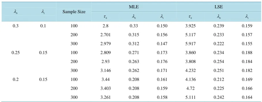
Table 1. Estimates of τ₀, λ₀, and λ₁ from simulated data.

0

λ λ1 Sample Size

MLE LSE

0

τ λ0 λ1 τ0 λ0 λ1

0.3 0.1 100 2.8 0.33 0.150 3.925 0.239 0.159 200 2.701 0.315 0.156 5.117 0.233 0.157 300 2.979 0.312 0.147 5.917 0.222 0.155 0.25 0.15 100 2.809 0.271 0.173 3.860 0.234 0.188 200 2.93 0.263 0.176 3.808 0.254 0.184 300 3.146 0.262 0.171 4.232 0.251 0.182 0.2 0.15 100 3.44 0.208 0.161 4.136 0.212 0.169 200 3.403 0.208 0.159 4.72 0.225 0.166 300 3.261 0.208 0.158 5.111 0.242 0.164

( )

(

,

( )

, 1

(

)

, 1, 2, ,

( )

1 ,

i i i

y t′ = f t y t y− t−τ i=  t∈ i− τ τi  (6)

with y₀

( )

t =g t

( )

. In brief, this idea is to shift the interval from _

( )

i−1 ,τ τi _ to _iτ,

(

i+1

)

τ_ and extend the

solution from

[

0,iτ

]

to _0,

(

i+1

)

τ_ by using the component in the current interval. This procedure can, in principle, be continued as far as desired. It is called, quite naturally, the method of steps [16].

Using the basic idea of the method of steps, first, we apply the DTM to find the solution to the following ODEs:

( )

(

( ) (

)

1 , 1 ,

y t′ = f t y t g t−τ

with t∈

[ ]

0,τ .

Suppose the approximate solution is given by

( )

[ ]

1 1

0

, 0,

k k k

y t a t t τ

∞

=

∑

∈

If τ >T, y t₁

( )

is the solution to (3). Otherwise, we should continue to find the solution in the interval

[

τ τ, 2

]

. At this time, we should solve the following ODEs

( )

(

( ) (

)

[

]

2 , 2 , 1 , , 2

y′ t = f t y t y t−τ t∈τ τ

Applying the DTM to the differential equation above again, we will obtain the following solution

( )

(

)

[

]

2 2

0

, , 2

k k k

y t a t τ t τ τ

∞

=

∑

− ∈

Of course, we should go on if 2τ <T holds also. In generally, applying the DTM to ODEs (6), we can obtain the analytic solution

( )

(

)

(

)

1 0

, , 1

k

n nk

k

y t a t nτ t nτ n τ

∞ +

=

∑

− ∈_ + _

until for some n, nτ< ≤T

(

n+1

)

τ. In fact, after necessary steps, we have the following solution to (3)

( )

[ ]

( )

[

]

( )

[

]

1

2

1

, 0, ,

, , 2 ,

, , .

n

y t t

y t t

y t

y t t n T

τ τ τ

τ

+

 ∈

 _∈

 =  

 _∈

(4)

Remark 1 If y t₁

( )

=g t

( )

, we can conclude that y=g t

( )

is the analytic solution to (3) directly.

Remark 2 If y_i₊₁

( )

t = y t_i

( )

for some integer i, we can conclude that the analytic solution (3) is

( )

[ ]

( )

(

) (

)

( )

(

)

1

, 0, ,

, 2 , 1 ,

, 1 , .

i

y t t

y t

y t t i i

y t t i T

τ

τ τ

τ

−

 ∈

 

=  _∈_ ₋ ₋ _

 



 _∈__ ₋ __





Remark 3 If we want to improve the accuracy of the approximate solution in each interval, we can combine the above method with the multi-step method given by[17].

Remark 4 In fact, the DTM based on the method of steps can also be applied to solve the following neutral delay differential equations

( )

(

( ) (

) (

)

( )

, , , , 0 ,

, 0.

y t f t y t y t y t t T

y t g t t

τ τ

 ′ = − ′ − ≤ ≤

 

= ≤



4. Numerical Experiments

In this section, four examples are given to show the performance of the DTM based on the method of steps. First, we want to solve the following simple but classical DDE to further illustrate the process of DTM.

Example 4.1 Consider the DDE [18]

( )

(

)

( )

1 , 0,

1, 1 0.

y t y t t

y t t

′

 = − − ≥



 ₌ _{− ≤ ≤}

 (7)

First, since τ =1, we apply the DTM to obtain the solution in the interval

[ ]

0,1 . In this interval, (7) can be

written as y t′

( )

= −1, and the initial condition is y

( )

0 =1. Taking the differential transform, we have

(

k+1

) (

Y k+ = −1

)

δ

( )

k , Y

( )

0 =1

It is easy to get

( )

1, 0,

1, 1,

0, 2.

k

Y k k

k

= 



= − =

 _≥



Thus we have the analytic solution y t

( )

= −1 t of (7) defined on [0,1].

Second, we should continue to solve the following DDE:

( )

(

)

( )

1 , 1 , 10 2,1,

y t y t t

y t t t

′

 = − − ≤ ≤



 _{= −} _{≤ ≤}



or equivalently,

( )

2 1

(

1 , 1

)

2

y t′ = − = − + −t t ≤ ≤t (8)

with initial condition y

( )

1 =0.

From (8), we have the following differential transform

(

k+1

) (

Y k+ = −1

)

δ

( )

k +δ

(

k−1 ,

)

Y

( )

0 =0 It is easy to get

( )

0, 0,

1, 1,

1

, 2,

2

0, 3.

k k Y k

k

= 

− =



=  ₌



 _≥

(5)

Thus we have the analytic solution

( )

(

) (

1

)

2

(

1

)

2

1 1 , 1 2

2 2

t t

y t = − − +t − = − +t − ≤ ≤t

Now, if we want to obtain the solution in the interval [2, 3], we should deal with the following DDE:

( )

(

)

( )

(

)

2

1 , 2 3,

1

1 , 1 2.

2

y t y t t

t

y t t t

′ = − − ≤ ≤

 

 −

= − + ≤ ≤

 

or equivalently,

( ) (

) (

2

)

2

2 , 2 3

2

t

y t′ = −t − − ≤ ≤t

with the initial condition

( )

2 1 2

y = − .

Then we have the following differential transform

(

) (

)

(

)

1

(

)

( )

1

1 1 1 2 , 0

2 2

k+ Y k+ =δ k− − δ k− Y = −

and get

( )

1

, 0,

2

0, 1,

1

, 2,

2 1

, 3,

6

0, 4.

k

Y k k

k

− =

 

= 



= =

 

− =

 

≥ 

Thus the analytic solution defined on [2, 3] is given by

( )

1

(

2

) (

2 2

)

3

(

1

) (

2 2

)

3

1 , 2 3

2 2 6 2 6

t t t t

y t = − + − − − = − +t − − − ≤ ≤t

The DTM can be proceed till the desire solution is obtained. Example 4.2 Consider the nonlinear DDE of third-order [11] [13]

( )

( ) (

)

( )

0.3

0.3 e , 0 1,

0 1, 0 1, 0 1, e , 0.

x

y x y x y x x

y f y y x x

− + −

′′′ = − − − + ≤ ≤

′ ′′

= = − = = ≤ (9)

Since τ =0.3, according to the foregoing, we have the following ODE, defined in the interval [0, 0.3]

( )

1 1

y′′′ x = −y x

Thus, applying DTM to the equation above, we obtain

(

k+1

)(

k+2

)(

k+3

) (

Y k+3

)

= −Y k

( )

The initial conditions lead to Y

( )

0 =1, Y

( )

1 = −1, and

( )

2 1 2

Y = . It is easy to have

( ) ( ) (

1 0

)

!

k

Y k k

k

−

= ≥ .

Thus we have the solution

( )

[

]

1

0 1

e , 0, 0.3 !

k

k x

k

y x x x

k ∞

−

= −

(6)

Noting that y x₁

( )

=g x

( )

=e−x, Remark 1 tells us y x

( )

=e−x is the analytic solution to (9) in the whole interval [0,1].

Remark 5 In [13], F. Karako and H. Bereketoğlu also apply DTM to DDE (9) where the initial function

( )

e x

y x = − , x≤0 is omitted, i.e.

( )

( ) (

)

( )

0.3

0.3 e , 0 1,

0 1, 0 1, 0 1, 0.

x

y x y x y x x

y f y x

− +

′′′ = − − − + ≤ ≤

′ ′′

= = − = ≤ (10)

It’s worth pointing out that, using the method given in [13], only approximate solution can be obtained. On the other hand, for DDEs (3), the initial function has the vital role. Without it, the DDEs may have un-unique

solution. In fact, Example 4.2 shows that y x

( )

=e−x is a solution to (10). Let’s suppose y x

( )

=e−x+f x

( )

is also a solution to (10), then f x

( )

should satisfy the following DDEs

( )

(

)

( )

0.3 , 0 1,

0 0 0 0, 0.

f x f x f x x

f f f x

′′′ = − − − ≤ ≤

′ ′′

= = = ≤ (11)

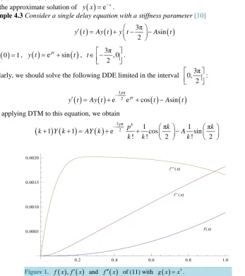
Figure 1 shows the solution to (11), together with it’s first and second derivative value on

[ ]

0,1 , with the initial function g x

( )

=x3, which satisfies the initial conditions in (10) obviously. It can be seen f x

( )

≠0,

then

( )

e x

( )

y x = − + f x is also the solution to (11). So, (11) has infinite solutions. Maybe, the authors “happen to” get the approximate solution of y x

( )

=e−x.

Example 4.3 Consider a single delay equation with a stiffness parameter [10]

( )

3π sin

( )

2

y t′ =Ay t +y t_ − _−A t

  (12)

with y

( )

0 =1,

( )

ept sin

( )

y t = + t , 3π, 0

2

t∈ −_ _

 .

Similarly, we should solve the following DDE limited in the interval 0,3π 2

 

 

 :

( )

_e 32π_e _cos

( )

_sin

( )

p pt

y t′ =Ay t + − + t −A t

Thus applying DTM to this equation, we obtain

(

₁

) (

₁

)

( )

_e 32π 1_cos π 1_sin π

! ! 2 ! 2

p k

p k k

k Y k AY k A

k k k

−    

+ + = + + _ _− _ _

[image:6.595.117.465.325.716.2]

   

Figure 1. f x

( ) ( )

, f′ x and f′′

( )

x of (11) with

( )

3

(7)

The initial values lead to Y

( )

0 =1. With the help of Mathematica, we have

( )

(

)

( )

3 π 3π

2 2

3 π 3 π 3π

2 2

2 2 2

3π

2 2 2

2

3π 3π 3π

2 3 2

2 2 2

3π

3 3 3

2

1 1

1 1 e e ,

1! 1! 1!

1 1 1

2 e e e

2 2! 2!

1

0 e ,

2! 2!

1

3 e e e

6

1 1

e ,

3! 3! 3!

p p

p p p

p

p p p

p

A A p

Y A

A p

Y A A p A A p

A A p

A p

Y A A Ap p

A A p

A p Y − − − − − − − − = + + = + + −   = _ + + _= + +   − = + + −   = _ − + + + _   − = − + + −

( )

3π 3 π

3 4 2 2 3

2 2

3π

4 4 4

2

3π 3π 3 π

4 5 3 2 2 3 4

2 2 2

3 π

5 5 5

2

3π 3 π

5 6 4 3 2 2 3

2 2

1

4 e e

24

1

0 e ,

4! 4!

1

5 e e e

120

1 1

e ,

5! 5! 5!

1

6 e e

720

p p

p

p p p

p

p p

A A A p Ap p

A A p

A p

Y A A A p A p Ap p

A A p

A p

Y A A A p A p A p

− − − − −   = _ + + + + _   − = + + −   = _ + + + + + + _   − = + + −

= + + + + 4 5

3 π

6 6 6

2 1

0 e ,

6! 6!

p

Ap p

A A p

A p −   + +       − = + + − 

Then, we obtain the solution to (12):

( )

(

)

3 π 3 5 2 0 0 3 π 2 0 0 3 π 2 1 e

1! 3! 5! ! !

e sin e

! !

e

sin e e e .

p

k k k

k k

p

k k

At k k

k k

p

At At pt

t t t A A p

y t t t

k k A p

A p

t t t

A p k k

t A p ∞ ₋ ∞ = = − _∞ _∞ = = −   − =_ − + + _+ + −     = + + _ − _ −   = + + − −

∑



This is the analytic solution to (12). Particularly, if

3 π 2 e

p

A= −p − , then the above solution can be simplified

to

( )

ept sin

( )

y t = + t , which coincides with the definition on 3π, 0 2

₋ 

 

 . So in this case,

( )

e sin

( )

pt

y t = + t

is the analytic solution to (12) in the whole interval

[

0,∞

]

.

As the last example, we apply the DTM based on the method of steps to solve a neutral delay differential equations.

Example 4.4 Consider the neutral delay differential equation

( )

(

1

)

( )

, 0 1

(8)

with the initial function y x

( )

=sin

( )

x , x≤0

According to the idea of the method of steps, DDE (13) becomes

( )

cos

(

1

)

( )

, 0 1

y x′ = x− −y x ≤ ≤x

Applying DTM to this equation, we have

(

) (

)

1 π

( )

1 1 cos 1

! 2

k

k Y k Y k

k

 

+ + = _ − −_

 

From the initial function, we get y

( )

0 =0, so Y

( )

0 =0. With the help of Mathematica, we have

( )

(

( )

)

( )

(

( )

)

( )

sin 1 1

1 cos 1 , 2 cos 1 sin 1 , 3 , 4 0,

2! 3!

cos 1 1 sin 1

5 , 6 cos 1 sin 1 , 7 , 8 0,

5! 6! 7!

cos 1 cos 1 sin 1 sin 1

9 , 10 , 11 , 12 0,

9! 10! 11!

Y Y Y Y

= = − + = − =

− +

= = = − =



Then, the solution to (13) is

( )

_{( ) (}

₎

(

( )

)

₍

₎

_{( ) (}

₎

( ) ( )

( )

(

( )

)

( )

(

)

(

)

(

)

4 1 4 2 4 3

0 0 0

cos 1 sin 1 cos 1 sin 1

4 1 ! 4 2 ! 4 3 !

sin sinh cos cosh sin sinh

cos 1 sin 1 cos 1 sin(1)

2 2 2

1 1

e sin 1 cos 1 cos 1 sin 1 .

2 2

k k k

x

x x x

y x

k k k

x x x x x x

x x

+ + +

+∞ +∞ +∞

= = =

−

= + − −

+ + +

+ − + − +

= + − −

= − + − − −

∑

5. Conclusion

Although the theory of differential transform method is not complete yet, it has been successfully applied to solve ordinary differential equations, partial differential equations, integral-differential equations, differential- algebraic equations and etc. In this paper, we apply DTM based on the method of steps to solve some delay differential equations, including neutral delay differential equations, successfully. Numerical experiments show that DTM is feasible and efficient for them. We believe that the operations of DTM presented in this paper also can be used to solve some partial delay differential equations (PDDEs), which is worth while studying in the future work.

Acknowledgements

This work is supported by the National Natural Science Foundation of China, contract/grant number 11371198 and 11401296, Jiangsu Provincial Natural Science Foundation of China, contact/grant no. BK20141008, Natural Science Fund for colleges and universities in Jiangsu Province contact/grant no. 14KJB110007, Jiangsu Provin- cial Key Laboratory for Numerical Simulation of Large Scale Complex Systems contract/grant number 201305 and 201401.

References

[1] Pukhov, G.E. (1986) Differential Transformations and Mathematical Modelling of Physical Processes. Naukova Dumka, Kiev.

[2] Zhou, J.K. (1986) Differential Transformation and Its Application for Electrical Circuits. Huazhong University Press, Wuhan. (In Chinese)

[3] Ayaz, F. (2004) Solutions of the System of Differential Equations by Differential Transform Method. Applied Mathe-matics and Computation, 147, 547-567. http://dx.doi.org/10.1016/S0096-3003(02)00794-4

(9)

International Journal of Computer Mathematics, 82, 369-380. http://dx.doi.org/10.1080/0020716042000301725

[5] Ayaz, F. (2004) Applications of Differential Transform Method to Differential-Algebraic Equations. Applied Mathe-matics and Computation, 152, 649-657. http://dx.doi.org/10.1016/S0096-3003(03)00581-2

[6] Liu, H. and Song, Y.Z. (2007) Differential Transform Method Applied to High Index Differential-Algebraic Equations.

Applied Mathematics and Computation, 184, 748-753. http://dx.doi.org/10.1016/j.amc.2006.05.173

[7] Abdel-Halim Hassan, I.H. (2002) On Solving Same Eigenvalue Problems by Using a Differential Transformation. Ap-plied Mathematics and Computation, 127, 1-22. http://dx.doi.org/10.1016/S0096-3003(00)00123-5

[8] Biazar, J., Eslami, M. and Islam, M.R. (2012) Differential Transform Method for Special Systems of Integral Equa-tions. Journal of King Saud University (Science), 24, 211-214. http://dx.doi.org/10.1016/j.jksus.2010.08.015

[9] Shadia, M. (1992) Numerical Solution of Delay Differential and Neutral Differential Equations Using Spline Methods. Ph.D. Thesis, Assuit University, Assuit.

[10] El-Hawary, H.M. and Mahmoud, S.M. (2003) Spline Collocation Methods for Solving Delay-Differential Equations.

Applied Mathematics and Computation, 146, 359-372. http://dx.doi.org/10.1016/S0096-3003(02)00586-6

[11] Evans, D.J. and Raslan, K.R. (2005) The Adomian Decomposition Method for Solving Delay Differential Equation.

International Journal of Computer Mathematics, 82, 49-54. http://dx.doi.org/10.1080/00207160412331286815

[12] Vanani, S.K. and Aminataei, A. (2008) On the Numerical Solution of Neutral Delay Differential Equations Using Mul-tiquadric Approximation Scheme. Bulletin of the Korean Mathematical Society, 45, 663-670.

http://dx.doi.org/10.4134/BKMS.2008.45.4.663

[13] Karako, F. and Bereketoğlu, H. (2009) Solutions of Delay Differential Equations by Using Differential Transform Me-thod.International Journal of Computer Mathematics, 86, 914-923. http://dx.doi.org/10.1080/00207160701750575

[14] Lainscsek, C. and Sejnowski, T.J. (2015) Delay Differential Analysis of Time Series. Neural Computation, 27, 594- 614. http://dx.doi.org/10.1162/NECO_a_00706

[15] Abazari, R. and Kilicman, A. (2014) Application of Differential Transform Method on Nonlinear Integro-Differential Equations with Proportional Delay. Neural Computing and Applications, 24, 391-397.

http://dx.doi.org/10.1007/s00521-012-1235-4

[16] Driver, R.D. (1977) Ordinary and Delay Differential Equations. Applied Mathematical Sciences, 20.

http://dx.doi.org/10.1007/978-1-4684-9467-9

[17] Odibat, Z.M., et al. (2010) A Multi-Step Differential Transform Method and Application to Non-Chaotic or Chaotic Systems. Computers & Mathematics with Applications, 59, 1462-1472. http://dx.doi.org/10.1016/j.camwa.2009.11.005