Strong convergence and bounded perturbation resilience of a modified proximal gradient algorithm

R E S E A R C H

Open Access

Strong convergence and bounded

perturbation resilience of a modified

proximal gradient algorithm

Yanni Guo

_{and Wei Cui}

*_{Correspondence:}

[email protected]

College of Science, Civil Aviation University of China, Tianjin, China

Abstract

The proximal gradient algorithm is an appealing approach in finding solutions of non-smooth composite optimization problems, which may only has weak convergence in the infinite-dimensional setting. In this paper, we introduce a modified proximal gradient algorithm with outer perturbations in Hilbert space and prove that the algorithm converges strongly to a solution of the composite

optimization problem. We also discuss the bounded perturbation resilience of the basic algorithm of this iterative scheme and illustrate it with an application.

Keywords: Strong convergence; Bounded perturbation resilience; Modified proximal gradient algorithm; Viscosity approximation; Convex minimization problem

1 Introduction

LetHbe a real Hilbert space with an inner product·,·and an induced norm · . Let 0(H) be the class of convex, lower semi-continuous, and proper functions fromH to (–∞, +∞]. Consider the following non-smooth composite optimization problem:

min

x∈H

f(x) +g(x), (1)

wheref,g∈0(H),f is differentiable and∇f isL-Lipschitz continuous onHwithL> 0. gmay not be differentiable. If further,f+g=:is coercive, that is,

lim

x→+∞(x) = +∞, (2)

thenhas a minimizer overH, that is,S:=Argmin()=∅, see [1, page 159, Proposi-tion 11.14]. Problem (1) has a typical scenario in linear inverse problems [2], it has ap-plications in compressed sensing, machine learning, data recovering and so on (see [3–6] and the references therein).

Proximal gradient methods are among the methods used for solving problem (1), which allow to decouple the contribution of the functionsf andg in a gradient descent step determined byf and in a proximal step induced byg [7, 8]. For the classical proximal gradient method, the initial valuex0∈His given, and the iterative algorithm for generating

sequence{xn}is defined as follows:

xn+1=proxλg(I–λ∇f)(xn), ∀n≥0, (3)

whereλ> 0 is the step size,prox_λgis a proximal operator (see Sect. 2). IfS=∅and 0 <λ<2_L, then any sequence generated by algorithm (3) converges weakly to an element of S[1, Corollary 27.9]. Xu [9] put forward the following slightly more general proximal gradient algorithm:

xn+1=proxλng(I–λn∇f)(xn) (4)

for problem (1), where the weak convergence of the generated sequence{xn}was obtained.

Besides, it was noted that no strong convergence is guaranteed ifdimH=∞. In 2017, Guo, Cui and Guo [10] proposed the following proximal gradient algorithm with perturbations:

xn+1=proxλng(I–λnD∇f+e)(xn). (5)

The generated sequence{xn}again converges weakly to a solution of (1).

On the other hand, it is well known that the viscosity approximation method proposed by Moudafi [11] generates a sequence{xn}:

xn+1=tnh(xn) + (1 –tn)Txn, (6)

which converges strongly to a fixed pointx∗ofTfor some contractive operatorh. In 2004, Xu [12, Theorem 3.1] further proved that the abovex∗is also the unique solution of the variational inequality:

(I–h)x∗,x–x∗≥0, ∀x∈Fix(T), (7)

provided that{tn}satisfies certain conditions.

This paper is based on viscosity algorithm (6) and proximal gradient algorithm (4) to generate a sequence with perturbations, which converges strongly to a solution of problem (1). We also apply this algorithm to solve the linear inverse problem.

1.1 Results and discussion

In view of the facts that the sequence generated by (5) converges weakly to a solution of (1), the viscosity method can convert a weakly convergent sequence to a strongly conver-gent one, and that the applied widely superiorization method introduced by [13] is based on the bounded perturbation resilience of basic algorithms, we discuss the strong conver-gence problem of a modified proximal gradient algorithm with perturbations as well as the bounded perturbation resilience of the responding basic algorithm.

The structure of this paper is as follows. In Sect. 2, we introduce some definitions and lemmas that will be used to prove the main results in the subsequent sections. In Sect. 3, we present the modified proximal gradient algorithm with perturbations and prove that the generated sequence{xn}converges strongly to a solution of problem (1). We conclude

this section with several corollaries. In Sect. 4, we introduce the definition of bounded per-turbation resilience and certify the corresponding strong convergence result. In Sect. 5, we apply our algorithm to the linear inverse problem, and illustrate it with a specific numer-ical example. Finally, we give a conclusion in Sect. 6.

2 Preliminaries

Let{xn}be a sequence in Hilbert spaceHandx∈H. LetT:H→Hbe an operator (linear

or nonlinear). We list some notations. xn→xmeans{xn}converges strongly tox.

xnxmeans{xn}converges weakly tox.

If there exists a subsequence{xnj}, which converges weakly to a pointz, we will callza

weak cluster point of{xn}. The set of all cluster points of{xn}is denoted byωw(xn).

Fix(T) :={x∈H:Tx=x}.

The following definitions are needed in proving our main results.

Definition 2.1 LetT,A:H→Hbe operators. (i) Tis nonexpansive if

Tx–Ty ≤ x–y, ∀x,y∈H.

(ii) TisL-Lipschitz continuous withL≥0, if

Tx–Ty ≤Lx–y, ∀x,y∈H.

We callTa contractive mapping if0≤L< 1. (iii) Tisα-averaged if

T= (1 –α)I+αS,

whereα∈(0, 1), andS:H→His nonexpansive. (iv) Aisv-inverse strongly monotone (v-ism) withv> 0, if

Ax–Ay,x–y ≥vAx–Ay2, ∀x,y∈H.

Giveng∈0(H), [1, Proposition 12.15] ensures thaty–x 2

Definition 2.2(Proximal operator) Letg∈0(H). The proximal operator ofgis defined by

prox_g(x) :=arg min

y∈H

y–x2 2 +g(y)

, x∈H. (8)

The proximal operator ofgof orderα> 0 is defined as the proximal operator ofαg. More-over, it satisfies (see [3, Remark 12.24])

prox_αg(x) :=arg min

y∈H

y–x2 2α +g(y)

, x∈H. (9)

The following lemmas (Lemma 2.3 and Lemma 2.4) describe the properties of the prox-imal operators.

Lemma 2.3([9, Lemma 3.1]) Let g∈0(H),andα> 0,μ> 0.Then

prox_αg(x) =prox_μg

μ αx+

1 –μ

α proxαgx .

Lemma 2.4([8, Lemma 2.4], [1, Remark 4.24]) Let g∈0(H),andα> 0.Then the prox-imity operatorprox_αgis1₂-averaged.In particular,it is nonexpansive,that is,

prox_αg(x) –prox_αg(y)≤ x–y, ∀x,y∈H. (10)

Lemma 2.5([9, Proposition 3.2]) Let f,g∈0(H),z∈H andα> 0.Assume that f is dif-ferentiable on H.Then z is a solution to(1)if and only if z solves the fixed point equation

z=prox_αg(I–α∇f)z. (11)

The following two lemmas play an important role in proving the strong convergence result.

Lemma 2.6 ([1, Theorem 4.17]) Let T : H →H be a nonexpansive mapping with

Fix(T)=∅.If{xn}is a sequence in H converging weakly to x,and if{(I–T)xn}converges

strongly to y,then(I–T)x=y.

Lemma 2.7([28, Lemma 2.5]) Assume that{an}is a sequence of nonnegative real numbers

satisfying

an+1≤(1 –γn)an+γnδn+βn, n≥0,

where{γn},{δn}and{βn}satisfy the conditions:

(i) {γn} ⊂[0, 1],

∞

n=0γn=∞,or equivalently,

∞

n=0(1 –γn) = 0;

(ii) lim sup_n→∞δn≤0;

(iii) βn≥0(n≥0),

_∞

n=0βn<∞.

3 Convergence analysis

In this section, letHbe a Hilbert space,h:H→Haρ-contractive operator withρ∈(0, 1). f,g∈0(H). f is differentiable, and∇f is Lipschitz continuous with Lipschitz constant L> 0. Givenx0∈H, we propose the following modified proximal gradient algorithm for solving (1):

xn+1:=tnh(xn) + (1 –tn)proxαng(I–αn∇f)(xn) +e(xn), n≥0, (12)

where{tn}is a sequence in [0, 1]. 0 <a=infnαn≤αn<2_L.e:H→Hrepresents a

pertur-bation operator and satisfies

∞

n=0

e(xn)< +∞. (13)

We also introduce the following iterative scheme as a special case to (12):

xn+1:=tnh(xn) + (1 –tn)proxαng(I–αn∇f+e)(xn), n≥0. (14)

We state the main strong convergence theorem.

Theorem 3.1 Let S be the solution set of(1),and assume that S=∅.Given x0∈H.Let{xn}

be generated by(12).If(13)and the following conditions hold: (i) 0 <a=infnαn≤αn<2_L,

∞

n=0|αn+1–αn|<∞;

(ii) {tn} ⊂(0, 1),limn→∞tn= 0;

(iii) ∞_n=0tn=∞,n∞=0|tn+1–tn|<∞.

Then {xn}converges strongly to a point x∗∈S, where x∗ is the unique solution of the

following variational inequality problem:

(I–h)x∗,x–x∗≥0, ∀x∈S. (15)

Proof We point out that prox_αng(I–αn∇f) is nonexpansive for each n. Let us follow

the proof of [29]. At first, that ∇f isL-Lipschizian means that∇f is 1_L-ism ([1, Theo-rem 18.15]). Consequently,I–αn∇f isα₂nL-averaged as 0 <αn<_L2([1, Proposition 4.33]).

Besides,prox_α

ng is

1

2-averaged by Lemma 2.4, the compositeproxαng(I–αn∇f) is

αnL+2

4 -averaged ([29, Proposition 3.2]). Then it is nonexpansive ([1, Remark 4.24]).

SetTn=proxαng(I–αn∇f). For anyx¯∈S, we have

Tnxn–x¯ ≤ xn–x¯

by applying Lemma 2.5 and thatTnis nonexpansive. So,

xn+1–x¯

=tnh(xn) + (1 –tn)Tnxn+e(xn) –x¯

≤tnh(xn) –x¯+ (1 –tn)Tnxn–x¯+e(xn)

≤tnρxn–x¯+tnh(x) –¯ x¯+ (1 –tn)xn–x¯+e(xn)

=1 –tn(1 –ρ)

xn–x¯+tn(1 –ρ)·

h(x) –¯ x¯

1 –ρ +e(xn)

≤max

xn–x¯,

h(x) –¯ x¯ 1 –ρ

+e(xn). (16)

An induction argument shows that

xn+1–x¯ ≤max

x0–x¯,

h(x) –¯ x¯ 1 –ρ

+ ∞

k=0

e(xk).

Hence{xn}is bounded as

∞

n=0e(xn)<∞. Consequently, we get the boundedness of

{h(xn)}and{Tnxn}.

We next prove thatxn+1–xn →0 asn→ ∞. In fact,

xn+1–xn

=tnh(xn) + (1 –tn)Tnxn+e(xn) –tn–1h(xn–1) – (1 –tn–1)Tn–1xn–1 –e(xn–1)

≤tn

h(xn) –h(xn–1)

+tnh(xn–1) –tn–1h(xn–1)

+(1 –tn)(Tnxn–Tnxn–1) + (1 –tn)Tnxn–1– (1 –tn–1)Tn–1xn–1 +e(xn)+e(xn–1)

≤tnρxn–xn–1+|tn–tn–1|h(xn–1)

+ (1 –tn)Tnxn–Tnxn–1+ (1 –tn)Tnxn–1–Tn–1xn–1 +|tn–tn–1|Tn–1xn–1+e(xn)+e(xn–1)

≤tnρxn–xn–1+|tn–tn–1|h(xn–1)+ (1 –tn)xn–xn–1 + (1 –tn)Tnxn–1–Tn–1xn–1+|tn–tn–1|Tn–1xn–1 +e(xn)+e(xn–1)

≤1 –tn(1 –ρ)

xn–xn–1+|tn–tn–1|h(xn–1)+Tn–1xn–1

+ (1 –tn)Tnxn–1–Tn–1xn–1+e(xn)+e(xn–1). (17) By applying Lemma 2.3 and Lemma 2.4, we compute

Tnxn–1–Tn–1xn–1 =prox_αng(I–αn∇f)

xn–1–

prox_α

n–1g(I–αn–1∇f)

xn–1 =prox_αng(I–αn∇f)

xn–1–proxαng

αn

αn–1

(I–αn–1∇f)xn–1

+

1 – αn αn–1

prox_αn–1g(I–αn–1∇f)

xn–1

≤(I–αn∇f)xn–1– αn

αn–1

(I–αn–1∇f)xn–1–

1 – αn αn–1

Tn–1xn–1

=1 – αn αn–1

xn–1–Tn–1xn–1

≤|αn–αn–1|

a xn–1–Tn–1xn–1, (18) wherea=infnαn> 0.

Substituting (18) into (17), we obtain

xn+1–xn

≤1 –tn(1 –ρ)

xn–xn–1+|tn–tn–1|h(xn–1)+Tn–1xn–1

+ (1 –tn)|

αn–αn–1|

a xn–1–Tn–1xn–1+e(xn)+e(xn–1)

≤1 –tn(1 –ρ)

xn–xn–1+|

αn–αn–1| a

xn–1+Tn–1xn–1

+tn(1 –ρ)·

(–1)· |αn–αn–1| a(1 –ρ)

xn–1+Tn–1xn–1

+|tn–tn–1|h(xn–1)+Tn–1xn–1

+e(xn)+e(xn–1)

≤1 –tn(1 –ρ)

xn–xn–1 +tn(1 –ρ)·

(–1)· |αn–αn–1| a(1 –ρ)

xn–1+Tn–1xn–1

+M1

|tn–tn–1|+|αn–αn–1|

+e(xn)+e(xn–1), (19)

where M1:=supn∈N{h(xn–1)+Tn–1xn–1,xn–1+_aTn–1xn–1} is well defined since {xn},

{h(xn)}and{Tnxn}are bounded.

By takingγn=tn(1 –ρ),δn=(–1)·|_aα_(1–n–ρα)n–1|(xn–1+Tn–1xn–1) andβn=M1(|tn–tn–1|+

|αn–αn–1|) +e(xn)+e(xn–1)in (19), we get

xn+1–xn →0, asn→ ∞ (20)

according to Lemma 2.7 and (i)–(iii) in Theorem 3.1.

Since{xn}is bounded, there exists a subsequence{xnj}such thatxnjzasj→ ∞. In

the sequel, we shall verify thatz∈S. To this end, assume thatαnj →α (j→ ∞), and set

T:=prox_αg(I–α∇f). We compute

xnj–proxαg(I–α∇f)xnj

≤ xnj–xnj+1+xnj+1–proxαg(I–α∇f)xnj

=xnj–xnj+1+tnjh(xnj) + (1 –tnj)Tnjxnj+e(xnj) –Txnj

≤ xnj–xnj+1+tnjh(xnj) –Txnj+ (1 –tnj)Tnjxnj–Txnj

+e(xnj). (21)

By using Lemma 2.3, we get

Tnjxnj–Txnj

=prox_α

=prox_αg

α αnj

(I–αnj∇f)xnj+

1 – α αnj

prox_α

njg(I–αnj∇f)xnj

–prox_αg(I–α∇f)xnj

≤ α

αnj

(I–αnj∇f)xnj+

1 – α αnj

prox_α

njg(I–αnj∇f)xnj

– (I–α∇f)xnj

=

α αnj

– 1 xnj+

1 – α αnj

prox_α

njg(I–αnj∇f)xnj

=1 – α αnj

xnj–Tnjxnj

≤1 – α αnj

·xnj+Tnjxnj

. (22)

Thus, we have

Tnjxnj–Txnj →0 asj→ ∞ (23)

in view of that{xnj},{Tnjxnj}are bounded forj, andlimj→∞αnj=α.

We combine (20), (21) and (23) to have

xnj–proxαg(I–α∇f)xnj→0 asj→ ∞, (24)

which implies thatz∈Sowing to Lemma 2.6, and henceωw(xn)⊂S.

Finally, we prove that

lim

n→∞xn–x ∗_{= 0.}

We have, by utilizing Lemma 2.4,

xn+1–x∗ 2

=tnh(xn) + (1 –tn)Tnxn+e(xn) –x∗2

=tn

h(xn) –x∗

+ (1 –tn)

Tnxn–x∗

+e(xn)2

≤tn

h(xn) –x∗

+ (1 –tn)

Tnxn–x∗2+ 2

xn+1–x∗,e(xn)

≤tn

h(xn) –x∗

+ (1 –tn)

Tnxn–x∗

2

+ 2xn+1–x∗e(xn)

=tn

h(xn) –h

x∗+ (1 –tn)

Tnxn–x∗

+tn

hx∗–x∗2

+ 2xn+1–x∗e(xn)

≤tn

h(xn) –h

x∗+ (1 –tn)

Tnxn–x∗

2

+ 2tn

hx∗–x∗,xn+1–e(xn) –x∗

+ 2xn+1–x∗e(xn)

≤tnh(xn) –h

x∗2+ (1 –tn)Tnxn–x∗

+ 2tn

hx∗–x∗,xn+1–e(xn) –x∗

+ 2xn+1–x∗e(xn)

≤tnρ2xn–x∗

2

+ (1 –tn)xn–x∗

2

+ 2tn

hx∗–x∗,xn+1–e(xn) –x∗

+ 2xn+1–x∗e(xn)

=1 –tn

1 –ρ2xn–x∗

2 + 2tn

hx∗–x∗,xn+1–x∗

– 2tn

hx∗–x∗,e(xn)

+ 2xn+1–x∗e(xn)

≤1 –tn

1 –ρ2xn–x∗2+ 2tn

hx∗–x∗,xn+1–x∗

+ 2tnh

x∗–x∗e(xn)+ 2xn+1–x∗e(xn)

=1 –tn

1 –ρ2xn–x∗2+ 2tn

hx∗–x∗,xn+1–x∗

+ 2tnh

x∗–x∗+xn+1–x∗e(xn)

≤1 –tn

1 –ρ2xn–x∗2+ 2tn

hx∗–x∗,xn+1–x∗

+M2e(xn), (25)

whereM2=supn∈N{2(tnh(x∗) –x∗+xn+1–x∗)}<∞in view oftn∈[0, 1] and{xn}being

bounded.

In order to apply Lemma 2.7 to (25), we need to prove

lim sup

n→∞

hx∗–x∗,xn–x∗

≤0. (26)

Select a suitable subsequence{xni}from{xn}such that

lim sup

n→∞

hx∗–x∗,xn–x∗

=lim

i→∞

hx∗–x∗,xni–x∗

. (27)

Since{xni}is bounded, it has a weakly convergent subsequence. Without loss of generality,

we denote the weakly convergent subsequence by {xni}and assume thatxniˆz. Then

ˆ

z∈S, and

lim sup

n→∞

hx∗–x∗,xn–x∗

=lim

i→∞

hx∗–x∗,xni–x

∗

=hx∗–x∗,zˆ–x∗

≤0. (28)

Takeγn=tn(1 –ρ2),δn=_1–2_ρ2h(x∗) –x∗,xn+1–x∗,βn=M2e(xn). Then all conditions

in Lemma 2.7 are satisfied. Thus

xn+1–x∗ 2

≤(1 –γn)xn–x∗

2

+γnδn+βn, (29)

which implies thatxn→x∗asn→ ∞.

Theorem 3.2 With the conditions in Theorem3.1hold,given x0∈H,the sequence {xn}

generated by(14)converges strongly to a point x∗∈S.

Proof We complete the proof by translating (14) into the form of (12). Indeed, we can rewritexn+1as

xn+1=tnh(xn) + (1 –tn)proxαng(I–αn∇f +e)(xn)

=tnh(xn) + (1 –tn)proxαng(I–αn∇f)(xn) +e(xˆ n), (30)

where

ˆ

e(xn) = (1 –tn)

prox_αng(I–αn∇f +e)(xn) –proxαng(I–αn∇f)(xn)

.

Obviously, ˆe(xn) ≤ e(xn) owing to Lemma 2.4 and tn ∈ [0, 1]. Thus we have

∞

n=0ˆe(xn)<∞. Since (12) was shown to converge, this immediately implies that (14)

converges strongly to a solution of (1).

If e(xn)≡0,n≥0, the exact form of the two modified proximal gradient algorithms

follows.

Corollary 3.3 With the conditions in Theorem3.1holding,and given x0∈H,arbitrarily, any sequence{xn}defined by

xn+1:=tnh(xn) + (1 –tn)proxαng(I–αn∇f)(xn), n≥0, (31)

converges strongly to a point x∗∈S.

We also get the following result of [12, Theorem 3.2] with T =prox_αg(I–α∇f) and αn≡α.

Corollary 3.4 With the conditions in Theorem3.1hold,given x0∈H,any sequence{xn}

defined by

xn+1:=tnh(xn) + (1 –tn)proxαg(I–α∇f)(xn), n≥0 (32)

converges strongly to a point x∗∈S.

In addition, ifhis some constant function, we have

Corollary 3.5 Under the conditions given in Theorem3.1,for any x0∈H,the sequence

{xn}defined by

xn+1:=tnu+ (1 –tn)proxαng(I–αn∇f)(xn), n≥0 (33)

4 Bounded perturbation resilience

The superiorization method can solve a broad class of nonlinear constrained optimal problems, which works by using the bounded perturbation resilience (BPR) of an origi-nal algorithm in order to steer the iterates of the algorithm towards to lower values of the objective function. In this paper, we investigate the BPR of the modified proximal gradi-ent algorithm. The superiorization version of this scheme will be presgradi-ented in the sequel paper.

Given a problem. Assume that we have a basic algorithm operatorA:H→H, where His a real Hilbert space. Then we have the following definition, which was originally given with a finite-dimensional Euclidean space [13].

Definition 4.1([14], Bounded perturbation resilience) An algorithmic operatorAis said to be bounded perturbation resilient if the following condition holds: if the sequence{xn},

generated byxn+1=Axnwithx0∈H, converges to a solution of, then any sequence{yn}

generated byyn+1=A(yn+βnvn) with anyy0∈H, also converges to a solution of, where the vector sequence{vn}∞n=0is bounded, and the scalars{βn}∞n=0are such thatβn≥0 for all

n≥0, and∞_n=0βn<∞.

If we treat the modified proximal gradient algorithm (31) as the basic algorithm A, the bounded perturbation of it is a sequence{xn}generated by

xn+1=tnh(xn+βnvn) + (1 –tn)proxαng(I–αn∇f)(xn+βnvn). (34)

We have the following result.

Theorem 4.2 Let H be a real Hilbert space.Let h:H→H be aρ-contractive operator,ρ∈ (0, 1)and f,g∈0(H).Assume the solution set S of(1)is nonempty.Assume,in addition, that f is differentiable,∇f is L-Lipschitz continuous on H.{βn},{vn}satisfy the conditions

in Definition4.1,{tn}and{αn}satisfy the conditions in Theorem3.1,respectively.Then any

sequence{xn}generated by(34)converges strongly to a point x∗in S.

Thus,the modified proximal gradient algorithm is bounded perturbation resilient.

Proof We rewrite (34) as

xn+1=tnh(xn+βnvn) + (1 –tn)proxαng(I–αn∇f)(xn+βnvn)

=tnh(xn) + (1 –tn)proxαng(I–αn∇f)(xn) +e(x˜ n), (35)

where

e(xn) =tn

h(xn+βnvn) –h(xn)

+ (1 –tn)

prox_α

ng(I–αn∇f)(xn+βnvn)) –proxαng(I–αn∇f)(xn)

.

In view of Lemma 2.4 and the assumptions as regardshandf, we have

e(xn)

≤tnβnvn+ (1 –tn)βnvn+αn

≤tnβnvn+ (1 –tn)(1 +αnL)βnvn

=1 + (1 –tn)αnL

βnvn, (36)

which implies that∞_n=0e(xn)<∞owing to the conditions imposed ontn,αn,βnand

vn. We then deduce the conclusion from Theorem 3.1.

5 An application and the numerical experiment

In this section, we apply Theorem 4.2 to linear inverse problem and show the numerical experiment.

5.1 Linear inverse problem

LetHbe a real Hilbert space andA:H→Ha bounded linear operator. Givenb∈H. We consider the following linear inverse problem:

Ax=b+w, x∈H, (37)

which is used to estimate an unknown signalxfrom the noise measurementbin finite-dimensional space.w is an unknown noise vector. This problem can be solved via the regularized least-squares problem:

min

x∈H

1

2Ax–b

2_+γx

, (38)

whereγ > 0 is a regularization parameter.

By applying algorithm (34) to (38), we obtain the following.

Theorem 5.1 Let h:H→H be aρ-contractive operator withρ∈(0, 1).Assume A= 0 and the solution set S of(38)is nonempty.Assume,in addition,{vn}is a bounded sequence

in H,{βn} ⊂(0, +∞)such that

∞

n=0βn<∞.Given x0∈H,we define{xn}by the iterative

scheme

xn+1=tnh(xn+βnvn) + (1 –tn)proxαnγ·

I–αnA∗

A(xn+βnvn) –b

(39)

(A∗is the adjoint of A),where (i) 0 <a≤αn<_A22,

∞

n=0|αn+1–αn|<∞;

(ii) {tn} ⊂(0, 1),limn→∞tn= 0;

(iii) ∞_n=0tn=∞,

∞

n=0|tn+1–tn|<∞.

Then {xn}converges strongly to a point x∗∈S, where x∗ is the unique solution of the

following variational inequality problem:

(I–h)x∗,x–x∗, ∀x∈S.

Proof Takef(x) = 1₂Ax–b2, g(x) =γx. It is easy to see thatf,g∈0(H),∇f(x) = A∗(Ax–b), and

_∇f(x) –∇f(y)

So∇f is Lipschitz continuous withL=A2_{. In addition,g is subdifferentiable, and its} subdifferential is

∂ · (x) =

⎧ ⎨ ⎩

{x/x}, ifx= 0;

B(0; 1), ifx= 0. (41)

So we can apply Theorem 4.2 to obtain this result.

5.2 Numerical experiment

In this subsection, we apply the iterative scheme (34) to solve (38) withH=RJ_to

demon-strate the effectiveness of this algorithm. For finite-dimensional spaces, the least-squares problem (38) takes the form as follows:

min

1

2Ax–b 2

2+γx1:x∈RJ

, (42)

where A∈RM×J is a matrix. The vector b∈RM. f(x) = 1₂Ax–b2₂ implies ∇f(x) = AT_{(Ax–b) with L=A}T_{A, where A}T _{represents the transpose ofA.prox}

αnγ·1(xn) = (prox_αnγ|·|

1(x 1

n), . . . ,proxαnγ|·|1(x

J

n))T, whereproxαnγ|·|1(x

k

n) =sgn(xkn)max{|xnk|–αnγ, 0},k=

1, 2, . . . ,J. The bounded sequence{vn}and the summarizable nonnegative real sequence

{βn}can be chosen as follows:

vn=

⎧ ⎨ ⎩

– dn

dn, if 0=dn∈∂g(xn),

0, if 0∈∂g(xn).

(43)

βn=cnfor somec∈(0, 1).

Throughout the experiments,A∈RM×Jis a matrix whose entries are sampled indepen-dently from a Gaussian distribution of zero mean and unit variance. The vectorb∈RM_is

generated from a uniformly distribution in the interval [–5, 5]. The regularization param-eterγ = 0.05. We chooseM= 50 andJ= 200. Giventn=₃1_n,αn=₃√_Ln_(n+1), we define the

stopping criterion

Err:=xn+1–xn<ε, (44)

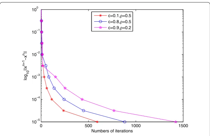
where ε is a given small positive constant. To see the behavior of algorithm (34), we plotted the evolutions of ‘Err’ defined by (44) with respect to the numbers of iterations in Fig. 1 for the initial point x0= (0, 0, . . . , 0)T∈R200. The plots in Fig. 1 show that the proposed algorithm is reliable to solve (42). Besides, The iteration numbers (“Iter”), the computing time in seconds (“Time”), the error’s values (“Err”) and (“Axn–b”) are

re-ported in Table 1 when the stopping criterionε= 5×10–5_{is reached. We can see from} Table 1 that the summarizable positive real sequence{β=cn}and the contractive con-stantρcan have a large impact on the numerical performance. We also find that the se-quence{xn}generated by algorithm (34) can get very close to the solution of the problem

Figure 1The numbers of iterations under the different error values

Table 1 Numerical results with different (c,ρ) and initial valuex0

(c,ρ) x0= (0, 0,. . ., 0)T _{x0= (1, 1,. . ., 1)}T

Iter. Time Axn–b Iter. Time Axn–b (0.1, 0.5) 152 0.140 0.066 199 0.140 0.074 (0.8, 0.5) 440 0.608 0.220 260 0.172 0.070 (0.9, 0.2) 680 0.546 0.307 773 0.484 0.353

6 Conclusion

In this paper, we introduced a modified proximal gradient algorithm with perturbations in Hilbert space by making a convex combination of a proximal gradient operator and a contractive operatorh. There exists a perturbation term in each iterative step (see (12)). We proved that the generated iterative sequence converges strongly to a solution of a non-smooth composite optimization problem. We also showed that the perturbation in com-puting the gradient off in algorithm (14) actually can be seen as a special case of (12). Finally, as one of the main objectives of this paper, we verified that the exact modified algo-rithm is bounded perturbation resilient, a fact which, to some extent, extends the horizon of the recent developed superiorization methodology.

Acknowledgements

The authors would like to acknowledge the reviewers for the very valuable comments which helped to improve the presentation of this paper. The authors also would like to acknowledge the National Natural Science Foundation of China (No. 11402294, 61503385) for financial support.

Competing interests

The authors declare that they have no competing interests. Authors’ contributions

All authors contributed equally and significantly to this paper. All authors have read and approved the final manuscript.

Publisher’s Note

Received: 15 September 2017 Accepted: 20 April 2018 References

1. Bauschke, H.H., Combettes, P.L.: Convex Analysis and Monotone Operator Theory in Hilbert Spaces. Springer, New York (2011)

2. Engl, H.W., Hanke, M., Neubauer, A.: Regularization of Inverse Problems. Kluwer Academic, Dordrecht (1996) 3. Bach, F., Jenatton, R., Mairal, J., Obozinski, G.: Optimization with sparsity-inducing penalties. Found. Trends Mach.

Learn.4, 1–106 (2012)

4. Daubechies, I., Defrise, M., De Mol, C.: An iterative thresholding algorithm for linear inverse problems with a sparsity constraint. Commun. Pure Appl. Math.57, 1413–1457 (2004)

5. Tibshirani, R.: Regression shrinkage and selection via the lasso: a retrospective. J. R. Stat. Soc., Ser. B, Stat. Methodol.73, 273–282 (2011)

6. Liu, Q.H., Liu, A.J.: Block SOR methods for the solution of indefinite least squares problems. Calcolo51, 367–379 (2014) 7. Lions, P.L., Mercier, B.: Splitting algorithms for the sum of two nonlinear operators. SIAM J. Numer. Anal.16, 964–979

(1979)

8. Combettes, P.L., Wajs, V.R.: Signal recovery by proximal forward-backward splitting. SIAM J. Multiscale Model. Simul.4, 1168–1200 (2005)

9. Xu, H.K.: Properties and iterative methods for the lasso and its variants. Chin. Ann. Math., Ser. B35, 501–518 (2014) 10. Guo, Y.N., Cui, W., Guo, Y.S.: Perturbation resilience of proximal gradient algorithm for composite objectives.

J. Nonlinear Sci. Appl.10, 5566–5575 (2017)

11. Moudafi, A.: Viscosity approximation methods for fixed-points problems. J. Math. Anal. Appl.241, 46–55 (2000) 12. Xu, H.K.: Viscosity approximation methods for nonexpansive mappings. J. Math. Anal. Appl.298, 279–291 (2004) 13. Censor, Y., Davidi, R., Herman, G.T.: Perturbation resilience and superiorization of iterative algorithms. Inverse Probl.26,

65008 (2010)

14. Censor, Y., Davidi, R., Herman, G.T., Schulte, R.W., Tetruashvili, L.: Projected subgradient minimization versus superiorization. J. Optim. Theory Appl.160, 730–747 (2014)

15. Censor, Y., Zaslavski, A.J.: Strict Fejér monotonicity by superiorization of feasibility-seeking projection methods. J. Optim. Theory Appl.165, 172–187 (2015)

16. Cegielski, A., Al-Musallam, F.: Superiorization with level control. Inverse Probl.33, 044009 (2017) 17. Garduño, E., Herman, G.: Superiorization of the ML-EM algorithm. IEEE Trans. Nucl. Sci.61, 162–172 (2014) 18. He, H., Xu, H.K.: Perturbation resilience and superiorization methodology of averaged mappings. Inverse Probl.33,

044007 (2017)

19. Helou, E.S., Zibetti, M.V.W., Miqueles, E.X.: Superiorization of incremental optimization algorithms for statistical tomographic image reconstruction. Inverse Probl.33(4), 044010 (2017)

20. Nikazad, T., Davidi, R., Herman, G.T.: Accelerated perturbation-resilient block-iterative projection methods with application to image reconstruction. Inverse Probl.28, 035005 (2012)

21. Schrapp, M.J., Herman, G.T.: Data fusion in X-ray computed tomography using a superiorization approach. Rev. Sci. Instrum.85, 053701 (2014)

22. Davidi, R., Censor, Y., Schulte, R.W., Geneser, S., Xing, L.: Feasibility-seeking and superiorization algorithm applied to inverse treatment plannning in rediation therapy. Contemp. Math.636, 83–92 (2015)

23. Censor, Y., Zaslavski, A.J.: Convergence and perturbation resilience of dynamic string averageing projection methods. Comput. Optim. Appl.54, 65–76 (2013)

24. Dong, Q.L., Zhao, J., He, S.N.: Bounded perturbation resilience of the viscosity algorithm. J. Inequal. Appl.2016, 299 (2016)

25. Jin, W., Censor, Y., Jiang, M.: Bounded perturbation resilience of projected scaled gradient methods. Comput. Optim. Appl.63, 365–392 (2016)

26. Nikazad, T., Abbasi, M.: A unified treatment of some perturbed fixed point iterative methods with an infinite pool of operators. Inverse Probl.33, 044002 (2017)

27. Xu, H.K.: Bounded perturbation resilience and superiorization techniques for the projected scaled gradient method. Inverse Probl.33, 044008 (2017)

28. Xu, H.K.: Iterative algorithms for nonlinear operators. J. Lond. Math. Soc.66, 240–256 (2002)