Towards a parameter free theory for electrochemical process at the nano scale

(1)

Towards a parameter-free theory for electrochemical process at the nano-scale

Ashwinee Kumar

Supervisor:

Prof. S. Sanvito Dr. C. CucinottaCo-Supervisor:

Department of Physics Trinity College Dublin

(2)

(3)

Declaration

I Ashwinee Kumar, hereby declare that this thesis has not been submitted as an exercise for a degree at this or any other university. It comprises work performed entirely by myself during the course of my PhD studies at Trinity College Dublin. I was involved in a number of collaborations, and where it is appropriate my collaborators are acknowledged for their contributions.

(4)

(5)

Abstract

(6)

(7)

Acknowledgements

I am indebted to many people for their help and guidance in the last 4 years.

First of all, I would like to thank my supervisor Prof. Stefano Sanvito for his continuous help, guidance and support during my PhD. His enthusiasm, insight into science and dedication to research have been an inspiration for me. Working under his supervision has been an incredible privilege. I would like to express my gratitude to Dr. Clotilde Cucinotta, from her I learned about the ab initio simulation of metal/water interfaces. Her input to this work through her ideas, insights and expertise is very much appreciated. Next, I would like to thank my lab mates - Maria, Mario, Yanhui, Emanuele, Urvesh, Rajarshi, Anais, Sabin for their constant help and support. I would especially like to thank Tom for the technical support and advice. I would also like to thank Stefania Negro, she was of great help in the starting of my PhD. I would also like to thank many friends from different societies especially DUHAC, they have been a great support from me in college. I would also like to thank TCHPC for providing me the computational power, and their staff members who all have been very helpful. I would also like to thank the Irish Research Council for providing the fund to carry out the research work.

(8)

(9)

List of Figures

1-1 A hydrogen fuel cell vehicle, which uses hydrogen as fuel and converts it into electricity. This in turn is used to drive the car, while leaving water as the combustion product [1]. . . 1

(14)

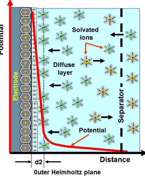
1-3 A simplified illustration of the Helmholtz double layer near the electrode-electrolyte interface. The electrode is positively charge, the electrode-electrolyte ori-ented with negative dipole towards it and solvated ions distributed inside the electrolyte. A steep decrease in the potential profile can also be observed within the double layer. ’d2’ marks the boundary of the DL (also known as outer Helmholtz plane), after that there is diffuse layer where diffusion of ions take place and further away to the right the seperator separates this layer from the bulk electrolyte [3]. . . 4 1-4 The STM image of D2O clusters on Pd(111) surface at 100 Kelvin. The

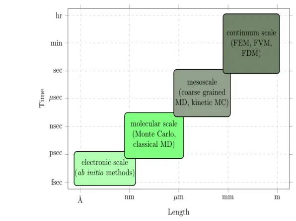
formation of hexagonal honeycomb clusters can easily be seen in this figure [4]. . . 5 1-5 Various materials modelling methods along with their associated time and

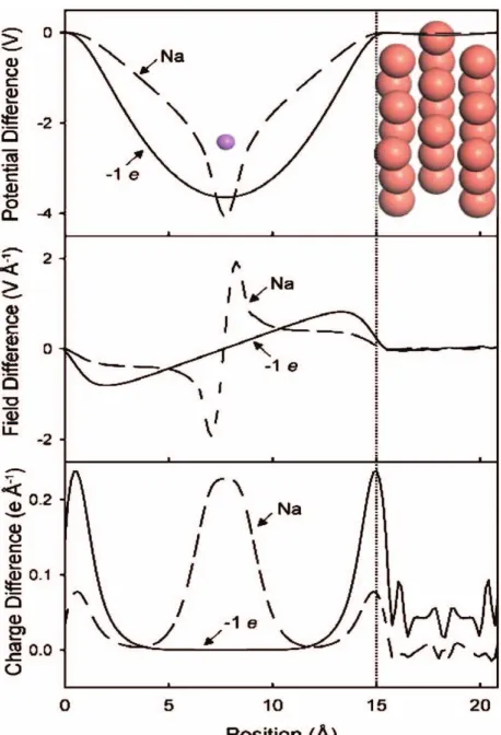
length scales. . . 7 1-6 Filhol and Neurock model showing the polarization of a bare Cu(111) slab

by either a sodium ion pseudopotential at the outer Helmholtz plane (Na) or the use of a continuum countercharge (1e), is illustrated by comparing plots of the electrostatic potential (top), electric field (center), and the change in electron density (bottom). Gradual decrease of electrostatic potential can be seen in top [5]. . . 10 1-7 Rossmeisl model showing a charged Pt(111) slab with 3 water layers

out-side and one solvated hydronium ion (yellow) per unit cell. The electrode potential, due to the charged interface and averaged parallel to the surface is shown for systems with 1, 2 and 3 relaxed water layers along with results [6]. . . 11

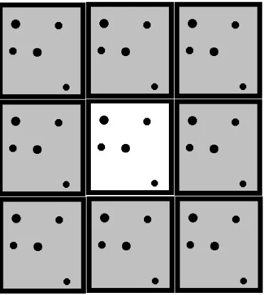
2-1 Figure showing a unit cell and different types of supercells in a 2D cubic crystal [7]. . . 21 2-2 Replication of the all atoms of white box throughout the space to form an

(15)

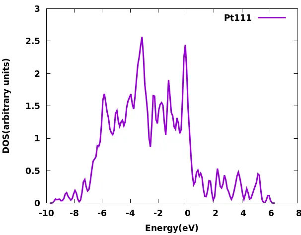
2-3 DOS of Pt(111) surface,the DOS does not have a HOMO-LUMO as it is a metal. Fermi level aligned with 0 eV. . . 24

2-4 PDOS of O and H of liquid water, shows separately the contribution of electron density of O and H. Fermi level aligned with 0 eV. . . 24

2-5 Figure shows the number of particles within a distance of𝑟and𝑟+𝑑𝑟(shown in green colour) away from the reference point (shown in blue colour) [8]. . 28

2-6 Figure shows the schematic energy level diagram for the calculation of work function in a metal. It is defined as the energy difference between the electrostatic potential in the vacuum and the Fermi level of the material (𝐸𝐹) [9]. . . 29

2-7 Figure shows different scenarios for substrate-molecule energy alignment. The solid substrate is depicted by red and blue colour for low and high work function respectively. The molecule is depicted by green colour and molecular levels are depicted by horizontal lines (two for HOMO and two for LUMO). Gray line at the intrerface represents lack of interface states,

∆ and 𝐸𝑇 are interface potential step and the tunneling barrier (defined

as the distance between the metal Fermi level and the molecular HOMO level) respectively. (A) Vacuum level alignment in the state of non electrical equilibrium. (B) Hybrid states (bonding groups) localised at the substrate-molecule interface, the interface can be polarised in order to maintain a net equilibrium between the electron chemical potential of the molecule (𝜇) and the fermi level of the solid (𝐸𝐹), this results in an extremely sharp induced

potential energy step (∆). (C) In cases where the substrate’s Fermi level

(16)

2-8 Single electron energy levels alignment and schematic picture of a Pt/electrolyte half-cell. 𝐸𝐹(Pt) separates filled and empty electronic states. Filled and

empty water molecular states lay well below and above 𝐸𝐹, respectively.

The highest occupied state for Na (here HOMO(Na), by analogy with the nomenclature for highest occupied molecular orbitals) is above𝐸𝐹, and thus

this species is expected to be fully ionised in solution. Correspondingly, the lowest unoccupied state for Cl, (namely, the degenerate Semi Occupied Molecular Orbital, SOMO(Cl)), is below 𝐸𝐹, therefore it becomes filled

in the system under consideration. Notably, a frozen picture of the single electron energy levels in our system is adopted here. . . 32

3-1 Figure showing energy vs 𝐾 points grid for bulk platinum showing the variation of total energy with variation in𝐾 points. . . 35 3-2 Figure showing energy vs lattice parameter at different 𝐾 points grid for

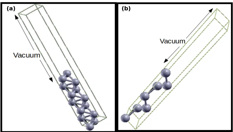
bulk platinum, used for optimizing the lattice parameter using the equation of states. . . 35 3-3 Figure shows the supercell of platinum used for modelling the 7 layers slab

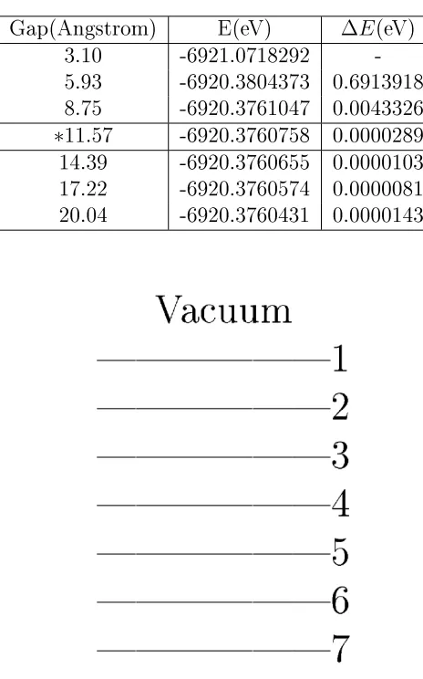
(a) (001) surface and (b) (111) surface. . . 37 3-4 The numbering of different layers of platinum with respect to vacuum,

start-ing with layer 1 from top to 7 at the bottom. . . 38 3-5 Figure shows the interlayer distance as a function of the 𝐾-points grid

(𝑋x𝑋x1) in Pt (001), it can be seen that as one moves from surface to centre the interlayer spacing comes closer to that of bulk. The convergence of the curves with increase in 𝐾 points can also be seen. . . 39 3-6 Interlayer distance as a function of K-points grid in Pt (111), it can be seen

(17)

3-7 PDOS of middle layer of 7 layers platinum surfaces (001) and (111) com-pared with bulk (surfaces calculated using 8X8X1𝐾points while bulk using 8X8X8 𝐾 points). It can be seen that the PDOS of (001) and (111) are all very similar to the bulk, so we conclude that they are able to mimic the property of the bulk to a large extent. . . 40

3-8 PDOS of symmetric layers(e.g 1 and 7, 2 and 6, 3 and 5 shown in figure (a), (b) and (c)) of the 7 layers Pt (001) slab compared with each other, the symmetric layers superimpose each other, confirming the same density of states (calculated with 8X8X1 𝐾 points grid). . . 41

3-9 PDOS of symmetric layer(e.g 1 and 7, 2 and 6, 3 and 5 shown in figure (a), (b) and (c)) of the 7 layers Pt (111) slab compared with each other, the symmetric layers superimpose each other, confirming the same density of states (calculated with 8X8X1 𝐾 points grid). . . 42

3-10 Work function vs K-points density Figure shows the work function as a function of the𝐾-points grid (𝑋x𝑋x1) in 7 layers Pt (a) (111) slab and (b) (001) slab. The convergence of the curves with increase in 𝐾 points grid can be observed. . . 43 3-11 PDOS of middle layer of 4 layers platinum surfaces (001) and (111)

com-pared with bulk Pt (surfaces calculated using 8X8X1𝐾 points while bulk using 8X8X8𝐾 points grid). . . 45

3-12 Interlayer distance as a function of K-points grid in Pt(001) 4 layers slab (calculated using 8X8X1 𝐾 points grid). Both the curves are showing a convergence behaviour with increasing𝐾 points grid. . . 45 3-13 Interlayer distance as a function of K-points grid in Pt(111) 4 layers slab

(18)

3-14 PDOS of symmetric layers(e.g 1 and 4, 2 and 3) of Pt(001) 4 layers slab compared with each other (a) PDOS of top and bottom layer (b) PDOS of both middle layer (both calculated using 8X8X1 𝐾 points grid). All the symmetric layers are superimposing on each other, confirming the symme-try. . . 46 3-15 PDOS of symmetric layer(e.g 1 and 4, 2 and 3) of 4 layers Pt(111) compared

with each other (a) PDOS of top and bottom layer (b) PDOS of both middle layer (both calculated using 8X8X1𝐾points grid). All the symmetric layers are superimposing on each other, confirming the symmetry. . . 47 3-16 Work function vs K-points density of a 4 layers Pt slab (a) for 4 layers

Pt(111) slab (b) for 4 layers Pt(001) slab (both calculated using 8X8X1𝐾 points grid). Both the curves are showing a convergence behaviour with increasing 𝐾 points grid. . . 47 3-17 Figure shows Pt/water solution model system. Here we present a snapshot

of the trajectory of the 0Na:0Cl system. Red, white and olive-green colour represent oxygen, hydrogen and platinum respectively. . . 48 3-18 0Na:0Cl system: graph of water density variation throughout the

elec-trolyte, it shows different region of water layers near the electrode i.g. first (min1) and second (min2) minimum of the water density profile. The sub-script ’l’ and ’r’ represent the left and right position of the respective minima. 49 3-19 Figure shows average atomic density profiles for the O and H atoms

(19)

4-1 Our Pt/water solution model system. Here we present a snapshot of the trajectory of the 10Na:12Cl system (with 10 Na and 12 Cl ions in solution). The horizontal bar on top of the snapshot marks the external boundary of the first and second water layer (𝑍1 and 𝑍2, respectively). 𝑍 = 0 labels

the average position of the surface Pt layers in contact with the aqueous electrolyte. Red, white, olive green, cyan and blue spheres represent O, H, Pt, Cl and Na atoms, respectively. . . 53

4-2 Average density profile of the O atom in the aqueous solution. To facilitate the reading, the results are vertically shifted. The separation between first and second water layer is identified by 𝑍1, while the separation between

the second region and the rest (bulk) of the solution is marked by the 𝑍2

interval, as the coordinate is not the same for the three interfaces. The zero of the Z scale is aligned to the position of the centre of the metal slab. . . . 58

4-3 10Na:12Cl system: graph of water density variation throughout the elec-trolyte, it shows different region of water layers near the electrode i.g. first minimum (min1), second minimum (min2) and shoulder of the water den-sity profile. The subscript ’l’ and ’r’ represent the left and right position of the respective label. It has the highest density of water in first layer compared to other two systems. . . 61

(20)

4-5 12Na:10Cl system: graph of water density variation throughout the elec-trolyte, it shows different region of water layers near the electrode i.g. first minimum (min1), second minimum (min2) and shoulder of the water den-sity profile. The subscript ’l’ and ’r’ represent the left and right position of the respective label. It has the least density of water in first layer clearly showing density dependense of water near the electrodes on the concentra-tion of ions in soluconcentra-tion. . . 63

4-6 Graphical representation of the overall excess (nominal-calculated) Bader valence charge distribution along the double layer. The charge is averaged along the trajectory and between the two surfaces present in our cell. The black dashed line (joining the Pt subsurface layers and the region in their middle) signals that in the middle of the metal slab the actual charge is 0 (see Fig. 4-10). . . 66

4-7 Effective potential drop, ∆𝑉, versus time for the three interfaces studied. The effective ∆𝑉 is obtained by subtracting from the electrostatic poten-tial of the total system (with charged electrode and electrolyte) that of its neutral separate components (i.e. the neutral electrode and the electrolyte, both surrounded by vacuum) in the same atomic configuration assumed in the charged system. . . 67

4-8 Absolute potential drop, ∆𝑉, versus time, for the three interfaces studied. The absolute ∆𝑉 is obtained as the difference between vacuum potential energy and the Fermi level. . . 68

(21)

4-10 Macroscopic total (ionic cores + valence electrons) charge (inset at the bottom, representation not to the scale) and electrostatic potential energy (top inset) profiles along𝑧(perpendicularly to the electrode surface), for the representative 10Na:10Cl system (represented in the central inset). These profiles are calculated along the trajectory every 1 ps (black lines). The average of these profiles is represented with a red line. Similar charge and potential drop trends are observed for all the systems. . . 70

4-11 Double layer charge versus potential drop∆𝑉 , as averaged along the trajec-tory for 12Na:10Cl (electrode charge -1.1 |𝑒|), 10Na:10Cl (electrode charge -0.6 |𝑒|) and 10Na:12Cl (electrode charge -0.03 |𝑒|) systems. Charge and potential drop are provided in units of |𝑒| and Volts, respectively. Also re-ported, the system’s capacitance (𝐶 = 8.29 𝜇F_·cm−2_{), evaluated from the}

(22)

4-12 Average atomic density profiles for the O and H atoms belonging to the aqueous electrolyte in contact with the electrode (in units of atoms per Å). 12Na:10Cl, 10Na:10Cl, and 10Na:12Cl systems are represented in black, red and blue, respectively. Differently unbalanced ion populations in solution lead to differently charged electrodes. The charge on the metal moiety of the interface is reported in the brackets next to each label (in units of |𝑒|). For each system, the atomic density profiles are averaged over 50 ps long trajectories obtained performing DFT based Born Oppenheimer molecular dynamics. First and second water layers are defined as described in Tab. 4.3. Here (a) represents the water molecules belonging to the first water layer, in contact with the electrode. In (b) the water molecules of the second water layer. The plain and dashed lines stand for the O and H atoms’ contributions, respectively. The separation between first and second water layer is identified by Z1, while the separation between the second region and

the rest (bulk) of the solution is marked by the Z2 interval. . . 74

4-13 Integrated O-H radial distribution profile (“Running” Coordination num-ber), where O belongs to the molecules of the first water layer in contact with the electrode. Black, red and blue lines represent the profiles relative to 12Na:10Cl, 10Na:10Cl and 10Na:12Cl systems, respectively. . . 75

(23)

4-15 Schematic view of the water bilayer at the Pt/H₂O interface for different state of charges (this is a cartoon showing the trend in the result, it’s not to the scale.). (a) Poorly charged Pt, typically with 10 Na and 12 Cl in solution, (b) negatively charge Pt, typically with 10 Na and 10 Cl in solution, (c) highly negatively charged Pt, typically with 12 Na and 10 Cl in solution. . . 77

4-16 Layer resolved surface sensitive vibrational density of states (VDOS), for 12Na:10Cl, 10Na:10Cl and 10Na:12Cl systems, represented with black, red and blue lines, respectively. The charge on the metal moiety of each DL is also reported in brackets, in units of |𝑒|. In (a) the VDOS obtained from the water molecules of layer 1, an increasing number of which points towards the bulk of the electrolyte, as the electrode becomes more positive. In (b) the VDOS obtained taking into account only water molecules of the second layer, where the number of water molecules reorienting their dipole towards the electrode becomes increasingly larger, as the electrode becomes more negative. . . 79

(24)

5-1 Comparison of the projected density of states (PDOS) on O, Cl and Na atomic species, for the 10Na:12Cl-Ag (blue) and 10Na:12Cl-Pt (green) sys-tems. The zero of the energy scale in these graphs is aligned to the Fermi level of the interface under consideration, so Cl and O PDOSes in Ag/water interface (upper inset) are lower in energy with respect to the Fermi level than those in Pt/water interface. This marks the lower value of Pt Fermi level with respect to vacuum. In the lower inset, the PDOS on Pt and the ions. A larger gap between Cl LUMO and Na HOMO is observed in the Ag/water interface. . . 84 5-2 Average density profile of the water in the electrolytic solution. The

sep-aration between first and second water layer is identified by Z1, while the separation between the second region and the rest (bulk) of the solution is marked by the Z2 interval. The shoulder is also clearly visible here similar to that of platinum electrode systems. The zero of the Z scale is aligned to the position of the centre of the metal slab. . . 87 5-3 Figure shows average atomic density profiles for the O and H atoms

be-longing to the aqueous electrolyte in contact with the electrode (in units of atoms per Å) for 10Na:12Cl-Ag system. Here (a) represents the water molecules belonging to the first water layer, in contact with the electrode. In (b) the water molecules of the second water layer. The plain and dashed lines stand for the O and H atoms’ contributions, respectively. Z1 and Z2 mark the end of the first and second layer. . . 88

6-1 Figure shows both the symmetric layer of the smaller system have sym-metric PDOS. In (a) PDOS of 1st and 4th layer of the smaller system is comapred and in (b) PDOS of 2nd and 3rd layer of the smaller system is compared. . . 94 6-2 Comparison of 2nd layer DOS of the smaller system, with that of the bulk

(25)

6-3 Figure shows the relaxation process of a 4 layer platinum (111) slab with 1 water molecule. It shows the orientation of the molecule at the beginning and end of the simulation (after relaxation), (a) shows top view of initial configuration, (b) shows top view of final configuration, (c) shows sideview of initial configuration and (d) shows sideview of final configuration. The red sphere represent the ’Oxygen’, white ’Hydrogen’ and olive green ’Plat-inum’. . . 96 6-4 Figure shows the relaxation process of 4 layer platinum (111) slab with 2

water molecule, it shows the orientation of the molecule at the beginning and end of the simulation (after relaxation), (a) shows top view of initial configuration, (b) shows top view of final configuration, (c) shows sideview of initial configuration and (d) shows sideview of final configuration. The red sphere represent the ’Oxygen’, white ’Hydrogen’ and olive green ’Plat-inum’. . . 97 6-5 Figure shows the relaxation process of 4 layer platinum (111) slab with 13

water molecule, it shows the orientation of the molecule at the beginning and end of the simulation (after relaxation), (a) shows top view of initial configuration, (b) shows top view of final configuration, (c) shows sideview of initial configuration and (d) shows sideview of final configuration. The red sphere represent the ’Oxygen’, white ’Hydrogen’ and olive green ’Plat-inum’. . . 98 6-6 Figure shows the relaxation process of 4 layer platinum (111) slab with 26

(26)

6-7 Figure shows the average potential profile of 4 layers platinum (111) surface on interaction with different number of water molecules- (a) potential pro-file of platinum with 1 water molecule on its surface, (b) potential propro-file of platinum with 2 water molecule on its surface, (c) potential profile of platinum with 13 water molecule on its surface and (d) Potential profile of platinum with 26 water molecule on its surface. . . 100 6-8 Variation of work function of Pt(111) with increasing number of water

molecule on its surface. . . 101 6-9 Distribution of water molecules on both side of Pt(111) surface, in new

smaller system. The middle layers of the slab are fixed. The red sphere represent the ’Oxygen’, white ’Hydrogen’ and olive green ’Platinum’ . . . . 103 6-10 Distribution of water density in smaller system, measured as distance from

the surface (surface=0Å) . . . 104 6-11 Average potential profile of Pt(111)-water (small system). The potential

shows uniformity on both side of platinum surface. . . 104 6-12 Charge variation in the small system, starting from the subsurface platinum

layer (SS), surface platinum (S), first layer of water (L1), second layer of water (L2), rest of water (RW). . . 105

7-1 Electrolytic cell in working condition [11, 12] . . . 112

A-1 Shown is the convergence of total energy as a function of force cutoff of a water molecule at a fixed box size. . . 114 A-2 Shown is the plot of variation of total energy of a water molecule as a

function of box size. . . 115 A-3 Shown is the graph of ∆𝐸 as a function of box size for the water molecule,

it can be seen that the ∆𝐸 fluctuates around 0 . . . 116 A-4 Shown are the charge density isosurface of the occupied molecular orbitals

(27)

A-5 Shown are the charge density isosurface of the unoccupied molecular orbitals of water starting from lowest energy (a) to highest (d). . . 118 C-1 The figure shows the solvations of anion (Cl) and cation (Na). It can be

easily seen that in the anion solvation shell ’(a)’ hydrogen of water molecules are pointing towards Cl, while in the cation solvation shell ’(b)’ hydrogen of water molecules are pointing away from Na. Due to the polar nature of water molecule it is behaving in such a way. . . 122 C-2 The figure shows the radial distribution function of different systems for

Cl-H. The first minima of G(r) curve is taken as cut off distance, defining the solvation shell. . . 122 C-3 The figure shows the radial distribution function of different systems for

(28)

(29)

List of Tables

3.1 Table showing the platinum lattice parameter and bulk modulus obtained by varying the 𝐾 points grid. . . 36 3.2 Total energy E and ∆𝐸 with variation in vacuum gap in 7 layers Pt(001).

The ’*’ marks the vacuum gap sufficient for modelling the surface. . . 37 3.3 Total energy E and ∆𝐸 with variation in vacuum gap in 7 layers Pt(111).

The ’*’ marks the vacuum gap sufficient for modelling the surface. . . 38 3.4 Interlayer distance in Platinum(001) using a 8x8x1 k point grid [(bulk

=1.995 Å)], it can be seen that symmetric layers have same interlayer distance. 43 3.5 Interlayer distance in Platinum(111) using a 8x8x1 k point grid [(bulk

=2.304 Å)], it can be seen that symmetric layers have same interlayer distance. 43 3.6 Total energy E and ∆ E as a function of the vacuum gap in a 4 layers

Pt(111) slab. . . 44 3.7 Total energy E and ∆ E as a function of the vacuum gap in a 4 layers

Pt(001) slab. . . 44

[image:29.612.114.560.223.705.2]

(30)

4.2 Excess Bader charges within the first solvation shell of Na ion. Water No., O, H and Water average represent the average number of water molecules, the average charge on O and H atoms, and on each water molecule in the first solvation shell around Na atom, respectively. Na+Water and Na represent the total average charge in each solvation shell and on Na ion, respectively. . . 56

4.3 Cartesian coordinates in Å used to define position and boundaries of first and second water layer. 𝑍𝑖 mark the external boundary of layer i and

correspond to the density minima of the O mass density profile. 𝑧𝑀 𝑖 mark

the position of the𝑖𝑡ℎ peak in the O mass density profile. All distances are measured from the Pt external surface layer . . . 57

4.4 Excess Bader charges in the first layer of water near the electrode. Water No., Total-Water, Avg.-Water, O and H represent the average number of water molecules, the total charge on the water layer, the average charge per water molecule, average charge per O and H atoms, respectively. . . 58

4.5 Excess Bader charges in the second layer of water near the electrode. Water No., Total-Water, Avg.-Water, O and H represent the average number of water molecules, the total charge on the water layer, the average charge per water molecule, average charge per O and H atoms, respectively. . . 58

(31)

4.7 10Na:12Cl system: comparison of water number density (per unit of cell surface) and excess Bader charges in the water layers near the electrode as calculated using either the minimum or the shoulder of the O density profile. Water No., Total-Water, Avg.-Water, O, H represent the average number of water in the first layer, total excess charge in the layer, average charge per water molecule, per oxygen and hydrogen atoms, respectively. . 60

4.8 10Na:10Cl system: comparison of water density and excess Bader charges in the water layers near the electrode as calculated using either the minimum or the shoulder of the O density profile. Water No., Total-Water, Avg.-Water, O, H represent the average number of water in the first layer, total excess charge in the layer, average charge per water molecule, per oxygen and hydrogen atoms, respectively. . . 60

(32)

4.10 Bader excess (nominal-calculated) valence charges in units of |𝑒|. In col-umn ‘system’, the name of the system under consideration, defined by the number of Na+ _{and Cl}– _{ions in solution and the type of metal electrode.}

In columns 2-6 the total, subsurface and external surface charge and the charge on first and second layer of water in contact with the electrode, re-spectively. These values are averaged along the trajectory and between the two interfaces present in our cell. Columns “Cl + H“ and “Na“ report the charge localised around Cl and Na ions. Due to the crude definition of the boundary of the volume defining the Bader charge around each atom, part of the charge actually localised on Cl was accounted by the Bader scheme to the charge of the H atoms pointing towards it. In this table the sum of Cl and this artificial H charges are reported. In the last two columns, “Solvation Shells“ and “DL“, we report the total charge in the first solva-tion shells of Na and Cl ions and the total charge on the double layer, DL, including electrode, first and second water layer. . . 64

4.11 Average number density of water molecules per surface in the cell and per system, in the first and second layer in contact with the electrode. The cross section of our cell is (A=286 Å2_{), corresponding to 42 surface Pt atoms. 75}

(33)

5.2 Excess Bader charges within the first solvation shell of Na ion. Water No., O, H and Water average represent the average number of water molecules, the average charge on O and H atoms, and on each water molecule in the first solvation shell around Na atom, respectively. Na+Water and Na represent the total average charge in each solvation shell and on Na ion, respectively. . . 89

5.3 Excess Bader charges in the first layer of water near the electrode. Water No., Total-Water, Avg.-Water, O and H represent the average number of water molecules, the total charge on the water layer, the average charge per water molecule, average charge per O and H atoms, respectively. . . 89

5.4 Excess Bader charges in the second layer of water near the electrode. Water No., Total-Water, Avg.-Water, O and H represent the average number of water molecules, the total charge on the water layer, the average charge per water molecule, average charge per O and H atoms, respectively. . . 90

(34)

5.6 Bader excess (nominal-calculated) valence charges in units of |𝑒|. In col-umn ‘system’, the name of the system under consideration, defined by the number of Na+ _{and Cl}– _{ions in solution and the type of metal electrode.}

In columns 2-6 the total, subsurface and external surface charge and the charge on first and second layer of water in contact with the electrode, re-spectively. These values are averaged along the trajectory and between the two interfaces present in our cell. Columns “Cl + H“ and “Na“ report the charge localised around Cl and Na ions. Due to the crude definition of the boundary of the volume defining the Bader charge around each atom, part of the charge actually localised on Cl was accounted by the Bader scheme to the charge of the H atoms pointing towards it. In this table the sum of Cl and this artificial H charges are reported. In the last two columns, “Solvation Shells“ and “DL“, we report the total charge in the first solva-tion shells of Na and Cl ions and the total charge on the double layer, DL, including electrode, first and second water layer. . . 91 6.1 Average distance of water molecules from Pt(111) surface in various sytem

before and after relaxation . . . 100 6.2 Excess of Bader charges in the first layer of the water near the electrode.

Water No., Total-Water, Avg.-Water, O and H represent the average num-ber of water molecules, the total charge on the water layer, the average charge per water molecule, the average charge per O and H atoms, respec-tively (for the small system). . . 102 6.3 Bader excess (nominal-calculated) valence charges in units of |𝑒| per unit

area of electrode in units of Å2_{, for electrode is compared under the section}

of Metallic electrode, then Interfacial water. Finally the number of inter-facial water molecules per unit area in units of Å 2_{, under the Water No.}

(35)

Chapter 1 Introduction

The study of the interface between water and other substrates is very important for under-standing the various processes taking place in biology, electrochemistry, fuel cell, battery, supercapacitor and more generally in science. There is a never-ending list of examples for the interaction of water with other substrates where surface interaction plays a crucial role.

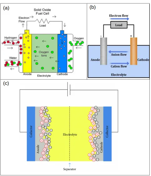
Figure 1-1: A hydrogen fuel cell vehicle, which uses hydrogen as fuel and converts it into electricity. This in turn is used to drive the car, while leaving water as the combustion product [1].

(36)

[image:36.612.165.406.66.347.2]

Figure 1-2: The working principles of different electrolytic devices. Panel (a) shows the working principle of a solid oxide fuel cell. Oxygen molecules turn into oxygen ions on coming in contact with the cathode. O ions travel to the anode through the electrolyte where they combine with hydrogen producing water. Panel (b) shows the working principle of a simple electrolytic cell. As soon as the electrodes are immersed in the electrolyte, the flow of anions to the anode and cations to the cathode begins, starting reduction and oxidation reactions at the respective electrodes and producing electricity in return. Panel (c) shows the working principle of superacapacitor (an irregular electrode can be seen over here, this is to increase the surface area of electrodes). The application of potential across the electrodes leads to anode and cathode covered with oppositely charged ions [2].

(37)

transfer, bond formation and bond breakage. It is described by the presence of long-range and short-range orders, hydrogen bonding and Van-der walls interaction. This system is very complex and difficult to study.

A successful model for the DL was first proposed by Helmholtz in 1853 [3]. He described the DL as a molecular dielectric which stores charge electrostatically (like a capacitor) independent of electrode charge density and dependent on dielectric constant of electrolyte. A simplified illustration of the Helmholtz double layer is shown in the Fig. 1-3. It clearly shows a steep potentail drop in the DL, a positively charged electrode and polarized electrolyte next to it. This model provides a good description of the interface but it did not consider the adsorption of ions on the surface of the electrode, the diffusion of ions in solution and the interaction between the solvent dipole moment and the electrodes.

Gouy-Chapman-Stern [13, 14] further modified Helmholtz model. They found out that the capacitance of the DL is not constant but vary with the application of the potential to the electrode as well as the ionic concentration. They also considered diffusion of the ions in the DL as well as adsorption on the electrodes. This model is the base of the study untill present day.

For decades these systems have been the subject of theoretical and experimental in-vestigations. Even with the rapid technological growth witnessed in the last few years the study of such interfaces has continued to interest the experimental and theoretical communities. There are many experimental techniques developed to study liquid-metal interfaces: low-energy electron diffraction (LEED), surface vibrational spectroscopies, such as surface enhanced Raman spectroscopy (SERS) and sum-frequency generation (SFG), high-resolution microscopy, like atomic force microscopy (AFM) and scanning tunneling microscope (STM), to name a few.

STM is a great tool for the study of surfaces, but it is not useful in ambient conditions since cryogenic temperatures and ultra-high vacuum are usually required to perform the experiments. Figure 1-4 shows a STM image of D2O clusters on Pd(111) at 100 Kelvin.

Clusters of D2O limited to few unit cell can be easily seen. Although this experiment

(38)

[image:38.612.161.405.82.380.2]

Figure 1-3: A simplified illustration of the Helmholtz double layer near the electrode-electrolyte interface. The electrode is positively charge, the electrode-electrolyte oriented with negative dipole towards it and solvated ions distributed inside the electrolyte. A steep decrease in the potential profile can also be observed within the double layer. ’d2’ marks the boundary of the DL (also known as outer Helmholtz plane), after that there is diffuse layer where diffusion of ions take place and further away to the right the seperator separates this layer from the bulk electrolyte [3].

(39)

[image:39.612.240.415.164.343.2]

From this short review we can appreciate the level of difficulty related to the under-standing of the double layer. A full underunder-standing will help us to take a step towards solving the energy and pollution problem of the world, by providing a clean and green source of energy, which is possible with the commercialization of fuel cells.

Figure 1-4: The STM image of D2O clusters on Pd(111) surface at 100 Kelvin. The

formation of hexagonal honeycomb clusters can easily be seen in this figure [4].

With the recent advances in computational techniques, the modelling of the interfaces is moving closer to realistic "liquid-water" interfaces. The best-suited theoretical tools to simulate these systems atomistic models, as they have turned out to be better for predicting experimental results [17]. They are even more useful for describing the processes occurring in extreme conditions of temperature and pressure [18]. Nowaday atomistic simulation are considered to be the best tool for the prediction of material properties, and for finding new materials for suitable processes. A large group of scientists is working to find new materials for aerospace, magnetism, elctrochemical applications using atomistic simulations [19].

1.1 My PhD work

(40)

in order to increase the energy output to fulfill the world energy demands. My study will mostly focus on the structure and properties of the double layer. Since, as already discussed, the formation of the double layer is the fundamental phenomenon occuring in an electrochemical environment. In particular we will look at the modeling of the electrostatic potential applied to the electrochemical cell at the molecular level. This can be used to monitor the reactions as well as developing better materials for water splitting [20]. Since there are different theoretical methods to model the double layer, it is very important to choose the appropriate one, which can predict the experimental phenomenon accurately. Many different types of modelling methods are available depending on the process to study. Each one of them has limitations and advantages, so the selection should be made carefully. Major issues in modelling the application of a potential to an interface are:

The size of the system (In atomistic simulations, depending on the type of system to equalize, it varies from thousands to tens of thousands of atoms. This is very far away from any practical system, a problem that is solved by using periodic boundary conditions (PBC) and supercells approach. These are disscussed in detail in chapter 2.)

Application of potential (Due to the implementation of PBC, to avoid the finite size effect, it is not possible to apply the potential directly to the electrode. In our model we will be using an imbalance population of ions in the electrolyte to charge the electrode, in turn applying the potential. This aspect will be discussed in detail in chapter 2.)

(41)

1.2 Choice of time scale

[image:41.612.163.461.203.425.2]

Figure 1-5 shows the various time and length scales addressed by the available theoretical tools. Accuracy is inversely proportional to the computational cost, so depending on the observable quantity a balance between accuracy and throughput should be reached before starting calculation of the selected system [21].

Figure 1-5: Various materials modelling methods along with their associated time and length scales.

(42)

to grouping of atoms, they also require some knowledge of the behaviour of the system in question prior to running the simulation. The required knowledge of the system can conveniently be extracted from ab initio or classical molecular dynamics results.

In the right corner there are the continuum-scale methods (e.g. finite-elements mod-elling (FEM), finite-volume method (FVM), finite-difference method (FDM)) [25]. At this scale the interactions between the electrons are incorporated indirectly using par-tial differenpar-tial equations. The resulting equations are coupled energy-balance equations, mass-balance equations and momentum-balance equations. These equations can be used to describe the transport of the constituting species by the means of conduction, convection and diffusion. These approaches are widely used in mechanical and civil engineering.

1.3 Literature Review

My work involves the study of the double layer equilibrium structure and the effects of an applied electrode potential. This will give me a deep insight into the structure and the reactivity of the interfaces and a comprehensive mechanistic description of the atomic and electronic scale processes at the electrode surfaces under an applied potential. Such understanding is still missing in the science community. Therefore, an ab initio approach is the best modelling method, which can be used. It has been already used for a long time [26, 27, 28] in modeling surfaces [29, 30, 31], but mostly focusing on reactivity of interfaces [32, 33, 34, 35, 36]. A comprehensive mechanistic description of atomic and electronic scale processes at the electrode surfaces under an applied potential is still missing. In particular, it is remarkable how limited our microscopic knowledge is of the double layer’s equilibrium structure and the effect of an applied electrode potential on it. This is true even for the most fundamental interfaces, such as Pt/water. Modelling the application of an external potential is a key challenge in the field of theoretical electrochemistry.

(43)

elec-trode and the other associated to the free electron. Excess/deficiency of charge can be introduced in the system by adjusting the surface potential and the method was used to analyse the case of Cu(111). Fig. 1-6 shows the variation of the charge and potential at the Cu(111) surface [5]. The problem of this method is that the potential drop is too grad-ual. This is not the case with the real electrolytic interfaces, where the potential drop is very sharp. However the method was successful in controlling the potential of the coupled interface system and in the introduction of fraction charge. Otani and Sugino [37, 38] tried to improve the model by introducing counter charges 15₋20Å in front of the electrode

surface, since most of the potential drop takes place outside the surface. Also this model was unable to correctly show the polarization of water at the interface. Rossmeisl [6] used a better approach by introducing a hydronium ion in the water layer outside the charged interface. In this way, the electrified interface is explicitly modelled. However, the ion is at a fixed distance from the electrode and no dynamical simulation of the double layer was performed. The Rossmeisl model is shown in the Fig. 1-7. This model was successful in constructing the energy diagram for the hydrogen evolution reaction at different potentials and it established the potential dependent nature of the reaction.

The potential drop at the interface is determined by several factors, such as the type of ions in solution and their dynamics, the work function of the metal, the surface charge density, the electric field at the interface and the polarizability. Most of the standard approaches achieve cell neutrality and the description of the potential drop at the interface. However, a reliable description of an electrified interface has yet to be obtained.

An alternative computational standard hydrogen electrode method, devised to inves-tigate coupled proton-electron transfer reactions, was developed by Sprik and co-workers [39, 40, 41]. This approach allows one to refer the computed potential to the standard hydrogen electrode (SHE) using the solvation free energy of the proton, calculated by measuring free energies from a common reference point, corresponding to the free energy of an aqueous hydronium ion H₃O+_{. The method is sophisticated and powerful, but its}

(44)

[image:44.612.171.400.69.405.2]

Figure 1-6: Filhol and Neurock model showing the polarization of a bare Cu(111) slab by either a sodium ion pseudopotential at the outer Helmholtz plane (Na) or the use of a continuum countercharge (1e), is illustrated by comparing plots of the electrostatic po-tential (top), electric field (center), and the change in electron density (bottom). Gradual decrease of electrostatic potential can be seen in top [5].

electrode method that avoids the expensive calculation of the solvation free energy of the proton has been introduced and applied to a few metal/water interfaces [35]. However, this does not include ions and does not address the problem of charging. Perhaps more importantly, it does not provide a description of the over-potential related to the transfer of species to, from or across the interface.

(45)

Figure 1-7: Rossmeisl model showing a charged Pt(111) slab with 3 water layers outside and one solvated hydronium ion (yellow) per unit cell. The electrode potential, due to the charged interface and averaged parallel to the surface is shown for systems with 1, 2 and 3 relaxed water layers along with results [6].

using simulations to reproduce reality and to carry out virtual experiments. In order to understand the electrolytic system thoroughly there is the need to address the problem by using a more comprehensive approach. In this approach we introduce imbalanced population of ions (e.g. 12Na:10Cl, 10Na:10Cl and 10Na:12Cl) in Pt-water system. They are expected to generate a charge of -1, 0 and +1 |e| on each electrode surface, respectively. This different status of charge will lead to the application of different potentials across the electrode, which will facilitate the study of the application of potential under PBC.

(46)

micro-scopic distance from the metal surface. However, none of them provides a realistic and self-consistent view of the structure and charge polarization within DL, able to capture the subtle interplay of electronic, ionic and thermal effects. This is due to the small size of the samples used and the lack of an extended dynamic description of its formation based on first principles. It has been experimentally proven [42] that the nature, structure and composition of the solvent at the interface with the electrode plays an essential role in de-termining its activity. Therefore a comprehensive modelling of the electro chemical (EC) environment overcoming traditional simplified models for the double layer, in combination with well-controlled experiment, is urgent and crucial to progress in the field. Here we present a realistic description from first principles of the Pt-water and Ag-water double layer structure and the charge distribution under an applied potential. In order to achieve this we have developed a general approach, which evolves previous methods towards a more comprehensive description of the metal/electrolyte interface. This is made possible as our model is extremely realistic and accounts explicitly and fully from first principles for charge polarization effects at both sides of the interface, the full dynamics of solvent rearrangment and electronic structures details. Besides unravelling for the first time the structure of the DL under an applied potential, our scheme also allowed us to directly evaluate the capacitance, the point of zero charge and the absolute electrode potential -by connecting the electrode Fermi level to the vacuum level and the standard hydrogen electrode. More in general, our approach also enables the estimation from first principles, the internal energy, the entropy and the free energies in a realistic environment. This information is also needed to develop and tune semi-empirical models able to simulate the steady state of large systems over time scales longer than those currently achievable with fully ab initio simulations.

(47)

Chapter 2 Theoretical tools and approximations

2.1 Methodological Approach

2.1.1 The Many-Body Problem

All the quantum mechanical properties of a system of𝑁 nuclei and𝑛 electrons can be, in principle, obtained by solving the many-body Schrödinger equations. The time indepen-dent non-relativistic Schrödinger equation is

ˆ

𝐻𝜓(𝑟,𝑅) =𝐸𝜓(𝑟,𝑅), (2.1)

where _𝐻ˆ _{is the Hamiltonian operator and} _𝜓₍_𝑟,_𝑅₎ _{is the many-body wave function. The}

solution of this equation depends on 3(𝑛+𝑁) interacting degrees of freedom (excluding

spin). More explicitly the Hamiltonian takes the form

ˆ

𝐻 = ˆ𝑇𝑒+ ˆ𝑉𝑖𝑜𝑛−𝑒𝑙+ ˆ𝑉𝑒𝑙−𝑒𝑙+ ˆ𝑇𝑖𝑜𝑛+ ˆ𝑉𝑖𝑜𝑛−𝑖𝑜𝑛, (2.2)

where,

ˆ

𝑇𝑒 =− ¯ℎ

2

2𝑚𝑒 ∑︀

𝑖∇

2

𝑖 is the kinetic energy operator for the electrons,

ˆ

𝑉𝑖𝑜𝑛−𝑒𝑙 =

∑︀

𝑖,𝐼 𝑍𝐼𝑒2

|𝑟𝑖−𝑅𝐼| is the operator for the electron-nuclei interaction, ˆ

𝑉𝑒𝑙−𝑒𝑙 = 1₂∑︀_𝑖̸=𝑗 𝑒2

(48)

ˆ

𝑇𝑖𝑜𝑛 =−

∑︀

𝐼

¯

ℎ2

2𝑀𝐼∇

2

𝐼 is the operator for kinetic the energy of nuclei,

ˆ

𝑉𝑖𝑜𝑛−𝑖𝑜𝑛 = 1₂∑︀_𝐼̸=𝐽

𝑍𝐼𝑍𝐽𝑒2

|𝑅𝐼−𝑅𝐽| is the operator for nucleus-nucleus interaction.

Hereℎ¯ is the reduced Planck’s constant, 𝑚𝑒,𝑒, 𝑟 are the mass, charge and position of

the electrons, while 𝑀, 𝑍, 𝑅are the mass, charge and position of the nuclei.

Solving the Schrödinger equation for3(𝑛+𝑁)interacting degrees of freedom is possible

only for the simplest model systems (e.g. where (𝑛+𝑁) is very small). However several

approximations have been developed to address the many-body problem.

The first simplification consists in the Born-Oppenheimer (BO) approximation, which allows one to separate off the nuclear degrees of freedom from the electronic ones. The BO approximation is based on the consideration that the mass of the nuclei is typically three to five orders of magnitude larger than that of the electrons, thus they move much slower. As a consequence their dynamics can be separated from that of the electrons [43]. The wavefunction of a system described by two independent variables can be written as the general solution of the Schrödinger equation 𝜓(𝑟,𝑅) = 𝜓(𝑟)𝜒(𝑅). Due to the

presence of the _𝑉ˆ

𝑖𝑜𝑛−𝑒𝑙 term it is not possible to express the wave function in this way.

However, it can be written in a general way 𝜓(𝑟,𝑅) = 𝜓(𝑟;𝑅)𝜒(𝑅), meaning that the

electronic component of the wave function, 𝜓(𝑟) depends on the nuclear coordinates.

Substituting 𝜓(𝑟,𝑅) =𝜓(𝑟;𝑅)𝜒(𝑅) in equation (2.1) allows us to separate the

elec-tronic equation from that of the nuclei. The elecelec-tronic wavefunction can be solved at a fixed positions 𝑅 for 𝑟. Solving for a range of 𝑅 gives the potential energy surface on which the nuclei move. The equation for the electronic part can then be written as

ˆ

𝐻𝑒𝜓(𝑟,𝑅) =𝐸𝑒𝑒(𝑅), (2.3)

where,

ˆ

𝐻𝑒 = ˆ𝑇𝑒+ ˆ𝑉𝑖𝑜𝑛−𝑒𝑙+ ˆ𝑉𝑒𝑙−𝑒𝑙. (2.4)

(49)

2.1.2 Hartree-Fock Approximation

Hartree proposed an approximation in 1927 in which he replaced the𝑛 electron wavefunc-tion 𝜓(𝑟𝑖)by a product of single-electron wavefunctions 𝜓𝑖(𝑟𝑖)

𝜓(𝑟1,𝑟2,𝑟3, . . . ,𝑟𝑛) =𝜓1(𝑟1)𝜓2(𝑟2)𝜓3(𝑟3). . . 𝜓𝑛(𝑟𝑛). (2.5)

The expression (2.5) is known as the Hartree product. In this the many electron problem is reduced to solving a one electron problem in the effective field generated by the other electrons. The Hartree product, however, fails to satisfy the antisymmetry principle, which states that a wavefunction describing fermions should be antisymmetric with respect to the interchange of any set of space-spin coordinates (𝑥). In order to take into account the spin, a new orbital is defined𝜒(𝑥= (𝑟, 𝛼)), related to 𝜓(𝑟) in the following way

𝜒(𝑥) =𝜓(𝑟)𝛼, (2.6)

where 𝛼 is a spin function. Using𝜒(𝑟), the Hartree product can be written as:

𝜓(𝑥1,𝑥2,𝑥3, . . . ,𝑥𝑛) =𝜒1(𝑥1)𝜒2(𝑥2)𝜒3(𝑥3). . . 𝜒𝑛(𝑥𝑛). (2.7)

Considering the two electron problem, the wavefunction which satisfy the antisymmetry principle can be written as

𝜓𝑠 =

1 √

(50)

Generalizing for𝑛 electrons gives the Slater determinant:

𝜓𝑠 =

1 (𝑛!)1/2

⃒ ⃒ ⃒ ⃒ ⃒ ⃒ ⃒ ⃒ ⃒ ⃒ ⃒ ⃒ ⃒ ⃒ ⃒

𝜒1(𝑥1) 𝜒2(𝑥1) 𝜒3(𝑥1) . . . 𝜒𝑛(𝑥1)

𝜒1(𝑥2) 𝜒2(𝑥2) 𝜒3(𝑥2) . . . 𝜒𝑛(𝑥2)

𝜒1(𝑥3) 𝜒2(𝑥3) 𝜒3(𝑥3) . . . 𝜒𝑛(𝑥3)

... ... ... ... ...

𝜒1(𝑥𝑛) 𝜒2(𝑥𝑛) 𝜒3(𝑥𝑛) . . . 𝜒𝑛(𝑥𝑛)

⃒ ⃒ ⃒ ⃒ ⃒ ⃒ ⃒ ⃒ ⃒ ⃒ ⃒ ⃒ ⃒ ⃒ ⃒

Expressing the wave function as a Slater determinant is equivalent to the assumption that each electron moves independently of all the others except that it feels the Coulomb repulsion due to the average positions of all electrons and it also experiences the exchange interaction due to antisymmetrization of the wavefunction. Some concepts of this de-scription also apply to Kohn-Sham density functional theory, which bears resemblance to Hartree-Fock theory.

2.1.3 Density Functional Theory (DFT)

DFT remaps the 𝑛-body problem into that of minimizing a functional depending on the electron density𝑛(𝑟). The electron density 𝑛(𝑟)is defined as the integral of the square of

many-body wave-function over all but one spatial coordinates of all electrons multiplied by the number of electrons.

𝑛(𝑟) = 𝑁

∫︁

. . .

∫︁

|𝜓(𝑟,𝑟1,𝑟2, . . . ,𝑟𝑛)|2𝑑𝑟1, . . . , 𝑑𝑟𝑛. (2.9)

This quantity depends only on 3 degrees of freedom. Contrary to the wave function, the electron density 𝑛(𝑟) is an observable and DFT establishes that this contains all

(51)

non-interacting electrons in a homogeneous electron gas [44].

Hohenberg-Kohn Theorems

Density functional theory is based upon two theorems given by Hohenberg and Kohn [45]-1. For a system of interacting particle in an external potential 𝑉𝑒𝑥𝑡(𝑟), the potential is

determined uniquely, except for a constant, by the ground state electron density𝑛𝑜(r).

2. A universal energy functional 𝐸[𝑛] of the density 𝑛(𝑟)can be defined, valid for any

external potential 𝑉𝑒𝑥𝑡(𝑟).

𝐸[𝑛] =𝑇[𝑛] +𝐸𝑖𝑛𝑡[𝑛] +

∫︁

𝑑3𝑟𝑉𝑒𝑥𝑡(𝑟)𝑛(𝑟) +𝐸𝑖𝑜𝑛−𝑖𝑜𝑛,

≡𝐹𝐻𝐾[𝑛] +

∫︁

𝑑3𝑟𝑉𝑒𝑥𝑡(𝑟)𝑛(𝑟) +𝐸𝑖𝑜𝑛−𝑖𝑜𝑛,

(2.10)

where: 𝑇[𝑛] is the kinetic energy of electrons and 𝐸𝑖𝑛𝑡[𝑛] is the total energy due to the

interaction among electrons. For any particular 𝑉𝑒𝑥𝑡(𝑟), the exact ground state energy of

the system is the global minimum of the functional, and the density 𝑛(𝑟) that minimizes

the functional is the exact ground state density 𝑛𝑜(𝑟) The Functional 𝐹𝐻𝐾 defined in

equation (2.10) includes all internal energy, kinetic and potential of the interacting electron system.

Kohn-Sham Scheme

In the Kohn-Sham approach the density-dependent problem is remapped onto an inde-pendent particle problem. This approach assumes that the total density of the original interacting system is equal to that of some non-interacting system subject to an effec-tive potential. The many-body contributions to the potential are incorporated in the exchange-correlation functional of the density 𝐸𝑋𝐶[𝑛]. The error is thus confined to the

approximation of the exchange-correlation functional [46]. The Kohn-Sham ansatz rests upon two assumptions:

(52)

an auxiliary system of non-interacting particles, which satisfies the equation

𝐻𝐾𝑆𝜙𝑖(𝑟) =𝜀𝑖𝜙𝑖(𝑟), (2.11)

where𝜙𝑖 is the single particle Kohn-Sham orbital and𝜀𝑖 are the Lagrange multipliers

that ensure the conservation of the number of particles.

2. The auxiliary Hamiltonian is chosen to have the usual kinetic energy operator and an effective potential 𝑉𝑒𝑓 𝑓 acting on the electrons,

𝐻𝐾𝑆 =−1₂∇2 + ˆ𝑉𝑖𝑜𝑛−𝑒𝑙[𝑛] +𝑉𝐻[𝑛] +𝑉𝑋𝐶[𝑛],

=₋1 2∇

2₊_𝑉

𝑒𝑓 𝑓[𝑛], (2.12)

where: 𝑉𝐻[𝑛] =

∫︀

𝑑3𝑟′_|𝑛_𝑟(₋𝑟_𝑟′)′_|, and 𝑉𝑒𝑓 𝑓[𝑛] = ˆ𝑉𝑖𝑜𝑛−𝑒𝑙[𝑛] +𝑉𝐻[𝑛] +𝑉𝑋𝐶[𝑛].

By using the Kohn-Sham approach the full interacting many-body problem can be written in the form

𝐸𝐾𝑆 =𝑇𝑒[𝑛] +

∫︁

𝑑𝑟𝑉𝑖𝑜𝑛−𝑒𝑙(𝑟)𝑛(𝑟) +𝐸𝐻[𝑛] +𝑉𝑖𝑜𝑛−𝑖𝑜𝑛+𝐸𝑋𝐶[𝑛], (2.13)

where: 𝐸𝐻[𝑛] =

∫︀

𝑑3_𝑟′_𝑑3_𝑟𝑛(𝑟)𝑛(𝑟′)

|𝑟−𝑟′_| ,

𝑇𝑒[𝑛] is the total kinetic energy of non interacting electrons and 𝐸𝑋𝐶 is the exchange

correlation energy.

2.1.4 Exchange-Correlation Functionals

A good approximation of 𝐸𝑋𝐶[𝑛] is important to obtain reliable results in DFT

calcu-lations. Unfortunately the exact exchange-correlation functional can be only found by solving the 3(𝑛 +𝑁) many-body wave function. The first attempt to find the explicit

(53)

that the exchange and correlation energy depend on the local value of density. This is called the local density approximation(LDA). The exchange-correlation functional can be written as:

𝐸_𝑋𝐶𝐿𝐷𝐴[𝑛(𝑟)] = ∫︁

𝑛(𝑟)𝜖𝑋𝐶(𝑛(𝑟))𝑑𝑟, (2.14)

where𝜖𝑋𝐶(𝑛(𝑟))is the exchange-correlation energy per particle of the homogeneous

elec-tron gas [47].

The LDA might look unrealistic but the results obtained with it are surprisingly good. However, LDA usually overestimates the binding energy (often of molecules and solids) and underestimates the bond lengths. The homogeneous electron gas is the only system for which the exchange-correlation functional is known and most of the functionals are based on this approach. One improvement over the LDA is the generalized gradient approximation (GGA), in which a dependence on the first derivative of the electron density is also included in the functional.

𝐸_𝑋𝐶𝐺𝐺𝐴[𝑛(𝑟)] = ∫︁

𝑓(𝑛(𝑟),_∇𝑛(𝑟))𝑑𝑟. (2.15)

Including the gradient gives better binding energy compared to the LDA. Many GGA parameterizations exist, differing in the functional form of the exchange and correlation energy. One of the most important functional form of 𝐸𝐺𝐺𝐴

𝑋𝐶 which has been used in this

work was developed by Perdew, Burke and Ernzerhof in 1996 (PBE) [48]. Some of the advantages of the PBE over the LDA are :

1. Atomic and molecular total energy are improved. 2. It gives better cohesive energy of solids.

3. Improved description of the relative stability of bulk phases. 4. More realistic for magnetic solids.

The LDA also has some advantages in a few cases over the GGA:

1. The LDA yields good relative bond energies for highly coordinated atoms, e.g. surface energies, diffusion barriers on surfaces.

(54)

LDA.

2.1.5 The Bloch Theorem

Until now our discussion was centered around dealing with the correlated nature of the electrons within a solid, but this is not the only problem. There are problems due to the large number of electrons in the solid. These can be overcome by considering that the whole electronic Hamiltonian and all the physical quantities describing a periodical system also share the translational invariance of the lattice. The Bloch theorem states that the single particle electronic wave function in a periodic crystal can be expressed in the form

𝜓𝑘(r) = eik.ruk(r), (2.16)

where 𝜓𝑘 is eigen states and 𝑢𝑘(𝑟) is a periodic function with the same periodicity of

the crystal e.g. 𝑢𝑘(r+Tn) =uk(r), whereTn is the periodic operator.

From the Bloch Theorem one can relate the periodicity in the potential with the periodicity in the wave function, e.g. for an infinitely periodic potential one does not need to solve the wave function over all the space, instead one can relate it to the periodicity in the wave function as shown in equation 2.16.

2.2 Computational Approach

2.2.1 Basis Sets Expansion

(55)

2.2.2 Supercells

In a perfect crystal, the atomic arrangement is in the form of a periodically repeated unit cell. Perfect periodicity is absent in many practical physical systems, but the system can be approximated to be periodic by choosing the necessary supercell. A supercell is a cell which consists of multiple units of the unit cell, it can be constructed in many different ways, such as the ones shown in figure 2-1. Few examples of systems where it is necessary to use supercells are point defects in crystals, surfaces and substitutional alloys. All these systems can be simulated by using the periodically repeated fictitious supercell. For example in the simulation of a point defect care should be taken that the defect does not interact with its image in order to simulate accurately the isolated defect. Surfaces are simulated by using crystal slab alternated with the slab of empty space taking care that the bulk behaviour is present in the centre of the slab and surface behaviour is unaffected by the presence of the periodic replica of the crystal slab. Finite systems too can be studied by using supercells. Enough empty space should be present between the periodic replica of the crystal slab so that the interaction between them is weak [7].

supercells

unit cell

(56)

2.2.3 Pseudopotentials

Valence electrons play a vital role in defining the physical and chemical properties of materials, while the core electrons do not have any significant role in the chemical bond. This fact can be utilized for simplifying the description of the atom. The pseudopotential is an effective potential constructed to substitute the all electron potential such that chemically active valence electrons are described by pseudo-wavefunctions while the core electrons being considered together with the nuclei by a suitably modified potential. The other desired property of pseudopotential is that it should be transferable (applicable to many different systems) [50], and as smooth as possible [51].

2.2.4 Periodic Boundary Conditions (PBC)

[image:56.612.193.379.396.604.2]

PBC enables the macroscopic properties of real systems to be calculated from a finite number of particles. The primary cell is replicated in all directions as image cells, the replica of the cells are called image cells. If the position of an atom in a simulation cell is

(57)

𝑟𝑖, then PBC also produces mirror images of the atoms of positions given by eq. 2.17

¯

𝑟𝑖𝑖𝑚𝑎𝑔𝑒= ¯𝑟𝑖+𝑙𝑎¯+𝑚¯𝑏+𝑛𝑐,¯ (2.17)

where 𝑎, 𝑏, 𝑐 are vectors that correspond to the edges of the box l, m, n are any integers from -∞ to +∞. Each particle is interacting with the particle in the box as well as the particles in the adjacent boxes. The choice of the origin of the simulation box has no effect on the behavior of the system.

Using the supercell approach and PBC the following rules should be taken into account: 1. The cell size should be sufficiently large to avoid the fictitious interaction of the

particles with their periodic images.

2. Any structural feature of the system of interest should be represented within the supercell.

2.2.5 Density of States (DOS)

One important concept in material science is that of the density of states (DOS). The density of states is defined as the number of energy states per unit volume per unit energy available to the system (the available states, which can be occupied by electrons). From the DOS one can understand the number of states available to be occupied by the electrons at a specific energy. For a system with a fixed volume, the DOS at a specific energy corresponds to the number of states available at that energy. The nature of adsorption of a molecule on a surface can be studied by investigating the changes of the DOS accompanied by the adsorption. The unit of the DOS is the number of states per volume of the supercell per eV. The DOS computed using DFT is most often reported in arbitrary units instead of its absolute value, since mostly the relative DOS values are of concern for many studies.

(58)

[image:58.612.127.430.89.326.2]

Figure 2-3: DOS of Pt(111) surface,the DOS does not have a HOMO-LUMO as it is a metal. Fermi level aligned with 0 eV.

[image:58.612.126.434.407.642.2]

(59)

unoccupied molecular orbital (LUMO). A valence band lies below the Fermi level and a conduction band lies above the Fermi level. The valence and conduction bands form two separate bands for semiconductors and insulators, and the energy gap between them is referred to as a band gap. A metal does not have a band gap and the Fermi level lies inside one band as shown in Fig. 2-3.

As DOS is useful in determining electron occupancy in specific energy level, it is often desirable to gain further insights such as which atom or orbital constitutes a particular energy level. A projected density of states (PDOS) helps one to determine the relative contributions of each orbital/atom to the total density of states at a given energy level. The DOS can be projected onto either an orbital or atom. Figure 2-4 shows the PDOS of O and H in liquid water.

2.2.6 ab initio Molecular Dynamics (AIMD)

(60)

wave function of the electrons is solved, so it clearly gives an upper hand to MD in terms of speed but AIMD can also incorporate effects due to bonding, charge transfer, polarization and many-body effects intrinsically, while in standard MD they must be imposed, artificially. In both methods, however, the motions of the atoms are computed by applying Newton’s second law to the atomic coordinates (by treating atoms classically). Quantum espresso and CP2K are the two plane wave DFT codes which I have used in my simulations.1

Initially, during the initialisation of the system (The initialisation of the system in-volved, finding the converged lattice parameter, work function, vacuum length on top of the platinum surface and interlayer distance between the layers of platinum surfaces), I have used Quantum espresso. Later for ab-initio molecular dynamics, CP2K is used (as ab-initio MD is not possible in Quantum espresso). I have double checked my earlier cal-culation in CP2K and found the same values as that of Quantum espresso (e.g. values of lattice parameter and work function of Platinum). Timestep and K point density plays a crucial role in DFT calculation, so, now we will discuss them next. Timestep and K point density plays a crucial role in DFT calculation, this will be discussed in detail in Appendix D. In the next section we will discuss QUICKSTEP [52], which is part of freely available computer code (CP2K), it performs accurate and efficient DFT calculations on large, complex systems. It has been used in our simulation to perform AIMD.

QUICKSTEP:

We present here the implementation of DFT method named QUICKSTEP, which is part of the freely available program package CP2K. New GPW (Gaussian Plane wave) method is implemented for fast and accurate calculation of DFT. GPW has been widely used for accurate DFT calculations in gas and condensed phases and can be effectively used for MD simulations. Although, the standard approach to DFT system was efficient and can handle hundreds of atoms. The DFT approach involved computation of the Hartree energy which in turn depends on the orthogonalisation of the wave functions which do not

(61)

scale linearly with the system size, and hence these terms dominate the computational cost of larger systems. The hybrid GPW which has been used in QUICKSTEP provides an efficient way to treat these terms accurately at a significantly reduced cost. In this method, the electron density is described by an auxiliary plane wave while atom-centred Gaussian type basis set is used to describe wave functions. Representation of density as plane wave improves the efficiency of Fast Fourier Transformation (FFT) as Hartree energy starts scaling linearly with system size. After defining the wave function next part as per the DFT calculation is the choice of pseudopotentials. In QUICKSTEP an extended database (H-Rn) with GTH pseudopotential parameters based on the local density approximation is available for use. It has also been optimised for use with an exchange-correlation potentials of Becke and Perdew (BP) [53], Becke, Lee, Yang, and Parr (BLYP) [53], Tozer and Handy (HCTH/120, HCTH/407) [54] and Perdew, Burke and Ernzerhof (PBE) [55].

Next part is the calculation of electrostatic energy which consists of contribution from electrons and nuclei. This is solved by using the Ewald sum method which treats all terms of electrostatic energy simultaneously (i.g. long range part of all electrostatic interactions is treated in Fourier space, whereas the short range is treated in real space). In the area of exchange and correlation, they did not find any method fully satisfactory, as a balance between the different accuracy goals is difficult to achieve. At last the accuracy of the system was tested by performing a test run on molecules (i.g. H2, Li2, LiH etc) to

calculate the bond distance and the results were compared with NUMOL (which L is a purely numerical DFT code and thus considered to be free of basis set effects). Results show a satisfactory agreement for all bond distances.

In summary, it can be said that the dual representation of charge density allows for an efficient treatment of Hartree energy terms in QUICKSTEP. Furthermore, the linear scaling of the Kohn-Sham matrix was obtained by the description of the wave function as a completely localised basis.