Using One Graph Cut to Fuse Multiple Candidate Maps in Depth Estimation

USING ONE GRAPH-CUT TO FUSE MULTIPLE

CANDIDATE MAPS IN DEPTH ESTIMATION

F. Piti´e

Sigmedia Group, Trinity College Dublin, [email protected]

Abstract

Graph-cut techniques for depth and disparity estimations are known to be powerful but also slow. We propose a graph-cut framework that is able to estimate depth maps from a set of candidate values. By employing a restricted set of candidates for each pixel, rough depth maps can be effectively refined to be accurate, smooth and continuous. The contribution of this work is to extend the graph structure proposed in the original papers on Graph-Cuts by Ishikawa and Roy, in such a way that sparse sets of candidates can be handled in one graph-cut.

Keywords:Graph-Cut, Depth Map Estimation,

1 Introduction

In 3D reconstruction from stereo, the problem of depth estimation can be thought of as a labelling problem. A convenient way of dealing with the labelling is to employ a Bayesian framework and consider that the depth map Dcan be modeled as a Markov Random Field (MRF). The interest of the Bayesian framework is that prior information on the spatial smoothness of the depth map can also be included. Typically, the energy of the MRF to be minimized will have the following form:

E(D) =X

p

Up(dp) +X

p,q

Vp,q(dp, dq) (1)

The functionUp(dp)is linked to the likelihood of having depth dpat pixelp. A small valueUp(dp)≈0means that this depth is very likely. The functionVp,q(dp, dq)is a smoothness penalty function, which essentially penalizes large difference of depth between neighbouring pixels.

This kind of energy has recieved a great deal of attention in recent years. Numerous optimization schemes have been proposed such as Simulated Annealing, Iterated Condition Mode, Belief Propagation, Tree Reweighted Message Passing or Graph-Cuts. In this paper we are interested in Graph-Cuts, a technique that has been used for some time now to solve smoothness constraints in labelling problems. The work of Ishikawa [2] and Roy [7, 6] brought graph cut to the attention of the computer vision community. The idea is to encode the likelihood and smoothness terms inside the capacities of a graph edges. The labelling is solved by finding a minimum cut through the graph. Each pixel is labelled as 0 or 1, depending on each side of the cut it lies. Graph-cuts have

been very successful at solving hard problems. They come however with some limitations since, in the general case, they can only solve the 2-labels problem. For n-labels, the general problem is believed to be NP hard and approximations to the exact solution must be considered. The works of Boykov, Kolmogorov and others have shown that with techniques such as alpha-expansion [1] and QPBO [5], n-labeling problems could be efficiently decomposed into a succession of 2-label problems.

A remarkable point in the original work of Ishikawa and Roy, is that an exact solution to a multi-labelling problem is however possible, with the caveat that the smoothness of the label field should be convex. For instance, the smoothness can follow the L1norm:

Vp,q(dp, dq) =αp,q|dp−dq| (2)

whereαp,q is a texture parameter, independent of the depth values. With this kind of penalty, Ishikawa [2] and Roy [7, 6] showed that it is possible to solve the multi-labelling by means of a minimum cut on a graph. The graph is of dimension width x height x number of labels. The depth likelihood and the spatial smoothness are encoded in the capacities of the graph edges. The labels can be extracted by cutting the graph, and reporting the edges that have been cut. Similar ideas have also been reported in more recent work such as Pariset al.[3] and it is also closely related to Total Variation [4], which offers a continuous framework to this problem.

Note that the convexity constraint on the smoothness terms has some important consequences. One issue is that solutions tend to minimize depth discontinuities. Thus large depth discontinuities can be over-smoothed. This can be mitigated by playing with the texture parameter αp,q, which can break the smoothness at image edges.

Contribution. The contribution of this paper is to provide a mechanism for solving Ishikawa and Roy’s graph using a sparse set of candidates. We argue that in most cases it is possible to obtain pretty good depth maps using fast but sub-optimal techniques, such as dynamic programming. Thus starting from a rough estimate, it is possible to propose for each pixel a set of a half dozen depth candidate that will contain the true depth value. Then, instead of working the full volume of disparities, we actually only need to consider a more manageable set of candidate values per pixel.

Using candidates in depth estimation is not a new idea. Woodford et al. [8] showed that depth maps can be fused using QPBO [5], an adaptation of the 2-label graph-cut technique. QPBO can only fuse two label fields; thus a number of iterations are required to refine the depth map. The advantage is that more complex smoothness model can be used and that the memory usage remains compact. The problem is the iterative nature of the method which leads to high computational times and convergence issues. We propose instead to start from the graph structure of Ishikawa and Roy’s graph and solve for multiple candidates at once and still obtain a global minimum. Our contribution is to provide a mechanism for setting up the weights in the reduced graph, in such way that the cut still yields a L1 _{norm smoothness}

between candidate values.

Organisation of the Paper. In the next section we describe Ishikawa and Roy’s graph structure. In section 3 we describe how the graph should be modified to accommodate candidate depths. The validity of the method is discussed in section 4 and practical results for depth estimation are presented in section 5.

2 Ishikawa’s and Roy’s Graph

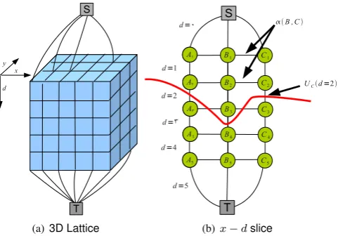
The graph structure presented in Ishikawa’s and Roy’s work is displayed in Fig. 1. Thexandyaxis of the graph correspond to the coordinates of the picture and thedaxis corresponds to the depth. Eachedgeof the graph corresponds one of the terms of the energy of equation (1). For thex-edges andy-edges, the capacity is given by the texture parameterαp,q between neighbouring pixelsp = (x, y)andq = (x0, y0). For the d-edges, the capacity isUp(d), the penalty for havingdat pixel

(x, y). Thus for a particular nodep= (x, y, d), the capacities of the incoming edges are given by:

(x, y, d)↔(x, y, d+ 1) = U(x,y)(d+ 1) (3)

(x, y, d)↔(x+ 1, y, d) = αp,q (4)

(x, y, d)↔(x, y+ 1, d) = αp,q (5)

For each pixel, the highest node (minimum depth) of the column is linked to a common special node (S), referred to as the source, and the lowest node (maximum depth) is linked to another special node (T), referred to as the sink:

(x, y, dmin)↔S = U(x,y)(d=dmin) (6)

(x, y, dmax−1)↔T = U(x,y)(d=dmax) (7)

AS −T cut of the graph separates the graph into two parts:

S

T d

y x

(a)3D Lattice

A1 A2 A3 A4 A5 B1 B2 B3 B4 B5 A1 A2 A3 A4 A5 C1 C2 C3 C4 C5 S T

d=0

d=2

d=1

d=3

d=4

d=5

UCd=2

 B ,C

(b)x−dslice

Figure 1: Regular lattice for the global graph cut minimisation. On the left, the 3D lattice of the graph. On the right, a 2D slice. The likelihood terms are reported on the vertical edges and the spatial smoothness penalty (x direction) is encoded in the horizontal edges. The minimum s−tcut gives the Maximum A Posteriori depth map, eg. in this casedA= 2,dB = 3anddC= 2.

one that includes the source S and one that includes the sink T. The sum of all edges that have been cut is actually the overall energyE(D)for the depth map. The depth map can be found by performing aminimum graph cut on this huge graph and reporting all the edges that have been cut as the depth for each pixel. For instance, after graph cut in Figure 1(b), the depth map for the three pixels isdA= 2,dB = 3anddC= 2.

To see that theL1 _{smoothness is induced, consider that after}

graph cut the depth isdA = 0and dB = 10. Then the 10 horizontal edges that are betweenA1andB10are cut. All these

edges have constant weightαA,B, thus the cut will have indeed a total cost of10αA,B=αA,B|dB−dA|.

3 Candidate Disparities

If finding the minimum cut is quite fast for small graphs, the method becomes unpractical for “very large” graphs. Typically, for image resolutions bigger than 300x300 pixels and a depth range greater than 60 values, graph cut will take a few minutes on modern CPU’s. Working with a subset of candidate disparities is thus an interesting alternative. Also, candidate depth values do not have to take integer values, thus by working with candidates we can obtain continuous depth maps.

In previous section graph structure, theL1penalty is induced by the “height” of each depth and thus the number of xand yedges that are cut. A similar mechanism can be used when dealing with candidates, albeit the weights for thexandyaxis will not be constant but will depend on the candidate values.

A5 A1 A2 A3 A5 B1 B2 B3

S

T

dA1=7

dA3=11.5

dA2=8.5

dA4=15

dB1=5

dB2=11

dB3=13

dB4=16

dA5=19

2 1.5 2.5 0.5 1.5 2 1 3

Cut=7.5=16−8.5

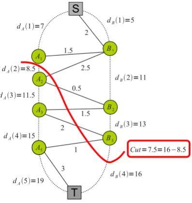
Figure 2: Example of a graph using candidate selection.

denoted as{dB(1),· · · , dB(4)}. Using the same setup as in Ishikawa and Roy, the graph comprises of 5-1=4 nodes for the pixel columnAand 4-1=3 nodes for the pixel columnB. Similarly the vertical edges correspond to the depth likelihood terms, eg. the edge (A1, A2) has a capacity of UA(dA(2)).

The weights for the edges between A and B have been set using the algorithm proposed hereafter. It is easy to verify that any cut will be proportional to the absolute difference of depths. Take for instance a graph cut (in red), which goes throughdA(2)anddB(4). The total cost for cutting thexand yedges is2.5 + 0.5 + 1.5 + 2 + 1 = 7.5, which is also the depth differencedB(4)−dA(2) = 16−8.5.

We propose in the following an algorithm that will automatically set these weights on the links between the AandB’s nodes.

3.1 Graph Construction.

It is sufficient to know how to connect two interacting pixels, since the same principle is then applied to all interacting pixel pairs. The construction of the graph is done in an iterative way. Consider the case of two pixelsAandBwith depth candidates {dA(i)}i≤NAand{dB(j)}j≤NB. To simplify the notations, we

define thatA0 = S = B0 andANA = BNB = T. Also we

notedA(i > NA) = +∞anddB(j > NB) = +∞.

Consider that after some iterations, A1,· · ·, Ai and

B1,· · · , Bjhave been connected (see Fig. 3). Denote

d0= min(dA(i+ 1), dB(j+ 1)). (8)

Ifd0 _=d

A(i+1)≤dB(j+1), then we add the edge(Ai+1, Bj) to the graph and we give it the capacity of

w=αA,B(min(dA(i+ 2), dB(j+ 1))−dA(i+ 1)) (9)

Conversely, ifd0 =dB(j+ 1)< dA(i+ 1), then we add the

Algorithm 1Setting up the smoothness edges for candidate disparities. Using notationsB(0) ≡ A(0) ≡ S,B(NB) ≡ A(NA)≡T anddA(i > NA) = +∞,dB(i > NB) = +∞.

i←0;j←0

while (i < NA)or(j < NB)do ifdA(i+ 1)≤dB(j+ 1)then

ConnectAi+1toBjwith edge capacity

c=αA,B[min(dA(i+ 2), dB(j+ 1))−dA(i+ 1)]; i←i+ 1;

else

ConnectBj+1toAiwith edge capacity

c=αA,B[min(dA(i+ 1), dB(j+ 2))−dB(j+ 1)]; j←j+ 1;

end if end while

edge(Ai, Bj+1)to the graph and we give it the capacity of

w=αA,B(min(dA(i+ 1), dB(j+ 2))−dB(j+ 1)) (10)

This process is summarized in Alg. 1.

3.2 Proof of Correctness

We need to show that any cut that goes through an edge

(Ap, Ap+1)and(Bq, Bq+1)will have a cost of the formC =

αA,B|dA(p+ 1)−dB(q+ 1)|.

To prove this we can proceed by recurrence. For two pixels A and B with disparities {dA(1),· · · , dA(NA)} and {dB(1),· · · , dB(NB)}, we assume that all the edges have been set, up toAiandBj.

Letd0 = min(dA(i+ 1), dB(j+ 1)). As illustrated in Fig. 4, consider a cut that goes through the edge(Ai, Bj)and exists through any other edge(Ap, Ap+1)or(Bq, Bq+1)with depth

d. Then the recurrence hypothesis is that the cost of cutting all the horizontal links between{A1,· · · , Ai}and{B1,· · ·, Bj} isC=αA,B|d0−d|. For instance in Fig. 4 (whereαA,B= 1), the orange cut that leaves the sub-graph at(S, B1)is assumed

to have a combined cost ofd0 −dB(1). Note that the edge capacity of(S, B1)is a likelihood edge, and is not included in

the horizontal edges.

If i = 0 and j = 0, then |dA(0)−dB(0)| = 0 and the recurrence hypothesis is satisfied.

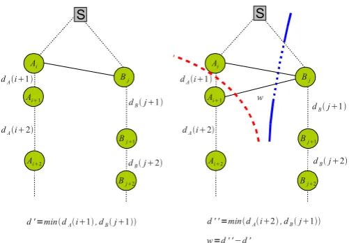
Without loss of generality, assume thatdA(i+ 1)< dB(j+ 1)

as in Fig. 3. Then,d0 =dA(i+ 1)and by construction,Ai+1

is connected toBj. Denoted00= min(dA(i+ 2), dB(j)). The capacity of the new edge is by constructionw = αA,B(d00− d0) = αA,B(d00−dA(i+ 1)). Consider now the recurrence hypothesis. A cut that goes trough(Ai+1, Bj)can either leaves

the subgraph by the nearby edge(Ai, Ai+1)or by an outer edge

of the previously built subgraph that corresponds to a depthd (see Fig. 3). In the first case, the cost of the cut will be onlyw=

S

dAi1

dBj1

Bj

Ai

d '=mindAi1, dBj1

Ai1

Bj1

dAi2

dBj2

Bj2

Ai2

S

dAi1

dBj1

Bj

Ai

Ai1

Bj1

dAi2

dBj2

Bj2

Ai2

w=d ' 'd ' w

d ' '=mindAi2, dBj1

Figure 3: Recurrence Steps. The graph has been connected up to the situation on the left. SincedA(i+ 1)<=dB(j+ 1), we connect Ai+1 to Bj. On the right, we can see that a cut going through(Ai+1, Bj)either leaves from(Ai, Ai+1) or from an edge higher than (Ai, Bj), in which case the Recurrence Hypothesis holds.

The cost is thenw+αA,B(d0−d) =αA,B(d00−d0+d0−d) = αA,B(d00−d). QEF.

4 Application to Depth Estimation Refinement

To show the interest of the technique, we start from a rough depth map, and refine the map by applying the global energy of equation (1) using depth candidates coming from the rough map. Here the initial depth map is estimated using Dynamic Programming (DP) along the scan line and using the normalized cross correlation over 3x3 blocks to build the likelihood. An example of such depth map is given in Fig. 5-(c). Since the optimization is done independently along scanlines, the resulting depth map suffers from heavy jitter artefacts.

We thus apply the model of equation (1) for a set of depth candidates generated from this initial depth map. In the first candidate pool, we consider the initial depth value for each pixel and add some of the neighboring depth values as candidates. The neighbouring candidates are taken as being the 8 most frequent depth values in a surrounding 50x50 block:

C1={d(x,y), d1F(x, y), d

2

F(x, y), d

3

F(x, y), d

4

F(x, y), d5_F(x, y), d6_F(x, y), d7_F(x, y), d8_F(x, y)} (11)

At the second iteration, the depth map is further refined by considering again some of the newly most frequent disparities plus extra variations:

C2={d(x,y), d1F(x, y), d

2

F(x, y), d

3

F(x, y),

d(x,y)+ 1, d(x,y)+ 2, d(x,y)−1, d(x,y)−2}

(12)

It is now easy to achieve a continuous map by iteratively

S

dA1

dAi1

dB3

dBj1

Bj

Bj

BAij

A1

A2

A3 BB_2j

Bj

B1

dB1

dB2

dA3

dA2

dA4

Cut=d '−dB1

Cut=d '−dA3

d '=mindAi1, dBi1

Figure 4: Recurrence Hypothesis. The sub-graph (solid lines) has been constructed up to nodes Ai and Bj. Let d0 _{= min(d}

A(i+ 1), dB(j + 1)). Consider a cut that goes through the edge(Ai, Bj)and exists through any other edge

refining these candidates.

C3={d(x,y), d(x,y)−.5, d(x,y)+.5, d(x,y)+.25,

d(x,y)−.25, d(x,y)−.75, d(x,y)+.75}

(13)

The texture parameters are defined to break the smoothness constraint at image edges. We chose the following edge aware model:

αp,q= 1

1 + 30kI(p)−I(q)k (14)

The difficulty of the method is to find the right candidates. If the right candidate is missing, then the method cannot recover. The results indicate however that candidates are rarely missed.

5 Results

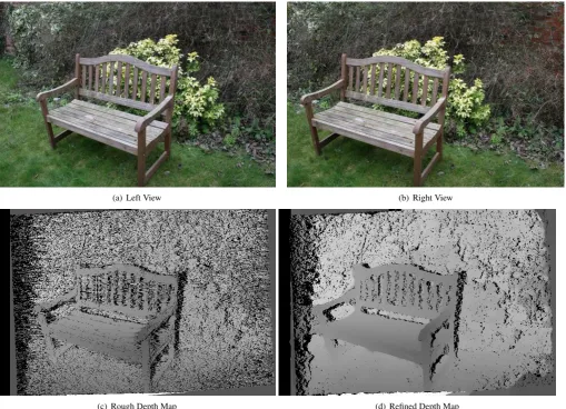
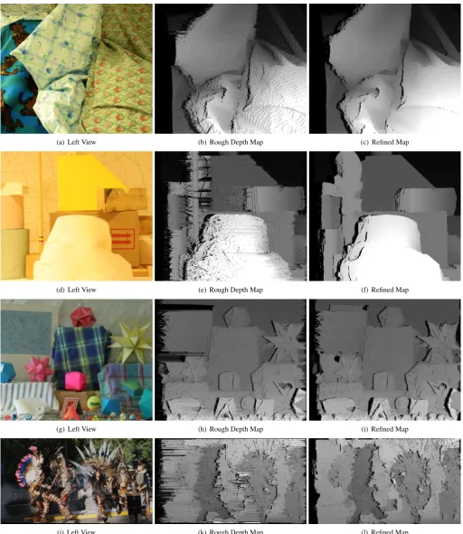
Results of the filtering process are displayed in Fig. 5 and Fig. 6. On Fig. 5 The left and right views are on top. On Fig. 6, the left column shows the left view image; the middle column the initial rough depth estimation; the refined map is on the right. Self-occlusions are displayed in black. Note that the refined map is visibly smoother and that the jitter artefacts have been completely removed. The quality of the results is however still essentially limited by the likelihood model, and oversmoothing of the depth map is sometimes noticeable across depth boundaries.

Comparison with full graph processing. On Fig. 7, we compare the candidate approach to using a full graph. On the right the results with using a full graph and on the left the results with the candidate approach described in this paper. The quality of both techniques is globally similar, although, on some places the candidate based approach displays some artefacts. These are due to a failure to pick up the correct disparity as a candidate. The candidate scheme has however a number of significant advantages: 1) it generates a subpixelic disparity map, 2) the computational effort is much lower.

On a 2.2GHz machine and using Kolmogorov’s implementation of maximum-flow/min-cut, graph-cut takes around a 2 seconds to process a 300x300 image block with 8 disparity candidates. Overall, including the DP pass, our technique takes around 25 second to process the 400x300 sequences. The computational time is independent of the number of disparities. The memory load is around tens of MB and is also constant.

With the full graph mincut, the processing time takes around 20 to 30 seconds for 20 disparities but for 60 disparities, the processing time raises to 2-3 minutes and the memory usage to 1GB. Dealing with higher resolution pictures and wider disparity range becomes quickly intractable.

6 Conclusion

We have presented an algorithm that allows to deal with non-regular values in Ishikawa’s and Roy’s graph. The graph

structure can be used to resolve depth estimation MRF’s energies for a sparse set of depth candidates. It offers thus an efficient framework to resolve multiple depth candidates per pixel at once in a reasonable amount of time. The drawback is that the smoothness penalty has to be convex and may oversmooth the depth map. We employed this technique to refine rough depth estimations obtained from using dynamic programming along scanlines. We showed that the method is very effective at improving the spatial smoothness of the rough estimates and can produce high quality continuous depth maps at a low computational cost.

A C++ implementation of the graph setup for sparse candidates is provided at www.sigmedia.tv/Publications/CVMP09/.

Acknowledgements

This work was funded by the FP7 European Project i3Dpost.

References

[1] Y. Boykov, O. Veksler, and R. Zabih. Fast approximate energy minimization via graph cuts. Pattern Analysis and Machine Intelligence, IEEE Transactions on, 23(11):1222–1239, Nov 2001.

[2] Hiroshi Ishikawa. Global optimization using embedded graphs. PhD thesis, New York, NY, USA, 2000. Adviser-Geiger, Davi.

[3] Sylvain Paris, Franc¸ois Sillion, and Long Quan. A surface reconstruction method using global graph cut optimization, February 2006.

[4] Thomas Pock, Thomas Schoenemann, Gottfried Graber, Horst Bischof, and Daniel Cremers. A convex formulation of continuous multi-label problems. In European Conference on Computer Vision (ECCV’08), 2008.

[5] C. Rother, V. Kolmogorov, V. Lempitsky, and M. Szummer. Optimizing binary mrfs via extended roof duality. InComputer Vision and Pattern Recognition, 2007. CVPR ’07. IEEE Conference on, pages 1–8, June 2007.

[6] S´ebastien Roy. Stereo without epipolar lines: A maximum-ow formulation.International Journal of Computer Vision, 34(2/3):147–162, August 1999.

[7] S´ebastien Roy and Ingemar J. Cox. A maximum-ow formulation of the n-camera stereo correspondence problem. InProceedings of the International Conference on Computer Vision, pages 492–499, January 1998.

(a) Left View (b) Right View

(c) Rough Depth Map (d) Refined Depth Map

(a) Left View (b) Rough Depth Map (c) Refined Map

(d) Left View (e) Rough Depth Map (f) Refined Map

(g) Left View (h) Rough Depth Map (i) Refined Map

(j) Left View (k) Rough Depth Map (l) Refined Map

(a) Tsukuba (b) Tsukuba

(c) Venus (d) Venus

(e) Teddy (f) Teddy

(g) Cones (h) Cones