Mass flow rate in gravity flow rig using optical tomography

www.arpnjournals.com

MASS FLOW RATE IN GRAVITY FLOW RIG USING OPTICAL

TOMOGRAPHY

Siti Zarina Mohd Muji1, Ruzairi Abdul Rahim2, Rahman Amirulah1, Norhidayati Podari1, Nurashlida

Ali1, Mohd Fadzli Abdul Shaib1

1_{Embedded Computing System (EmbCoS) Focus Research Group, Department of Computer Engineering,} Faculty of Electric and Electronics Engineering, Universiti Tun Hussein Onn Malaysia (UTHM), Parit Raja,

86400 Batu Pahat, Johor, Malaysia 2

Department of Control and Instrument, Faculty of Electrical Engineering, University Teknologi Malaysia, 81310 Skudai, Johor, Malaysia

E-Mail: szarina@uthm.edu.my

ABSTRACT

Monitoring mass flow rate is important in solid gas application. There are two common technique namely, inferential and direct method. Direct method is the focus in this research as it only involves in single plane system. The optical tomography system will be placed at the gravity flow rig to find its percent of concentration, and this value will be manipulated to get the mass flow rate. Direct method is the solution for a system that needs easy computation.

Key words: Mass Flow Rate, Gravity Flow Rig, Optical Tomography, Direct Method

INTRODUCTION

In solid gas industries such as pharmaceutical, agriculture (grain and rice), animal feed pellets, food(flour, sugar, tea, coffee), mining and quarrying (lump coal, crushed ores mineral), oil industry (barytes, cement , bentonite used for drilling purpose) and glass manufacture (sand), a mass flow rate is an important indicator for monitoring the solid flow. All of these involve whether a gravity flow rig or pneumatic flow rig. However, the fact is measuring a mass flow rate is not an easy job because many factors will affect the measurement and result in an incorrect measurement of mass flow rate. Among the factor that affect the mass flow rate correctness are inhomogeneous solid distribution, irregular velocity profiles, variable particle size, moisture content and other parameters (Yan,1996). Until now, only few of mass flow rate meter are accepted in industry, and some effort must be done to develop a mass flow rate meter. The mass flow rate can be measured whether using an inferential or direct method. Research has been done to measure the mass flow rate measurement in a variety of tomography technique such as using electrostatic sensor by Tajdari and Rahmat (2011) and electrodynamic tomography by Rahmat et. al. (1997). Both techniques have success in measuring mass flow rate. A complete review on the issue involves in mass flow rate measurement can be reviewed in Zheng and Liu (2010). The inferential method using optical tomography has been investigated by Pang (2004), and Chiam (2006) and they used a concept of multiplying the velocity parameter with a percentage of concentration. The drawback for inferential method is, it involves heavy computation and needs very fast processing time to make sure the measurement of mass flow rate can be done. 30 frame per second are the range for the lowest value that can be considered as fast processing time for dynamic

give an extra work in the mass flow rate measurement. Among the researcher that used a direct method are Yingna Zheng et. al. (2006), Abdul Rahim et. al. (2008) and Yunus (2005). Yingna Zheng et. al. used an equation that involves gravity value, where they assume the gravity value is the same for all the measurement taken. While for Abdul Rahim and Yunus there is no gravity value that involve, where there only find a calibration value from a graph of mass flow rate versus percentage of concentration.

This research will refer a technique produced by Abdul Rahim and Yunus with a different method in getting the image reconstruction. In our research the technique to get the image reconstruction is based on the combination between fan beam and parallel beam projection.

The paper will be divided into five elements. First is about introduction, second will focus on the method involve in the measurement of mass flow rate, thirdly will involve result and discussion; fourthly is the conclusion for overall works.

THE GRAVITY FLOW RIG OPERATION

The research to get the mass flow rate is done using gravity flow rig in the lab. The system layout is depicted in Figure 1. To operate this flow rig, below is the procedure

1) The main switch will be activated

2) Then the vacuum loader switch will be ON. Here the plastic beads will be sucked into the hopper via a barrel.

Figure 1: Gravity Flow Rig

The Calibration Process

Before doing the mass flow rate measurement, a calibration needs to be done. Calibration means to check, adjust, or determine by comparison with a standard (the graduations of a quantitative measuring instrument). The standard value for the gravity flow rig is get from measurement of the weight of the particles that go trough the flow rig divided with the time taken for the particles to drop fully in the tank. Previous research by Alias (2002) measured a mass flow rate by fixing the time to 15 second and measure the weight of the particles. Yunus (2005) using the same technique by adding a flow indicator for every time the particle is measured.

In the case of a flow rig that has an inhomogeneous flow, the system need to be tuned to the maximum speed, in order to provide accurate reading. Therefore the flow indicator needs to adjust to high value to form the calibration graph. The low value of the flow indicator cannot produce a needed graph because the graph produced is not a linear one. By using the greater value of flow indicator, the flow that is produce is higher and therefore the mass flow rate will give a right value according to the baffle openings. While for the low value of flow indicator, the particle that flow is likely the same for all baffle opening as the flow cannot give the different value for different baffle size. Figure 2 shows the graph using low value of flow indicator.

Figure 2: The mass flow rate value using different baffle for 20 Hz flow indicator

As shown in Figure 2, the calibration graph that form by 20Hz flow indicator cannot give a linear relation therefore the equation that produce from this graph cannot be used for mass flow rate equation. Therefore a higher value will be used to get the linear calibration graph as shown in the next section. The calibration data will form a calibration graph and the equation that intercept the origin will be used along with concentration value to get the mass flow rate.

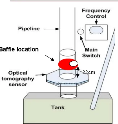
Experiment Setup

The baffle will be inserted at the bottom of the pipe which is near to the sensing area. The reason for the location is to avoid any gravity effect that will involve if the baffle location is far apart from the sensing element. It means that, the near the baffle to the sensing element, the result of the mass flow rate calibration is directly proportional to the opening of baffle area and do not have any outside effect such as collision with pipe wall or bouncing and other factor that can influence the measurement.

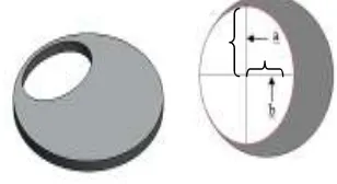
Table 1 shows 9 different size of baffle; 10%, 20%,30%,40%, 50%, 60%,70%,80% and 90%. Each baffle correspond to concentration percentage. To calculate the baffle opening area, equation (2) can be used as it has elipse shape (Garmer, 2007). Figure 3 shows the baffle that will be used in this research and Table 1 shows the calculation for the opening ellipse at nine different baffles as mentioned.

2

2













=

d

A

π

π

×

×

=

a

b

B

%

100

)

(

×

=

A

B

P

where,

A = Area of the baffle while full opening B = Area of opening ellipse at the baffle

P = Concentration percentage of the flow inside pipeline

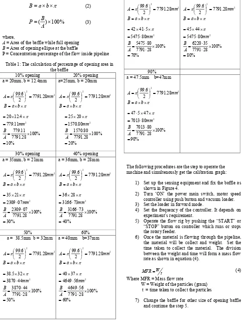
Table 1: The calculation of percentage of opening area in the baffle

10% opening 20% opening

a = 20mm, b = 12.4mm 2 2 28 . 7791 2 6 . 99 mm

A  =

     =π π × ×

=a b

B % 10 % 100 28 . 7791 11 . 779 11 . 779 4 . 12 20 2 = × = = × × = A B mm π

a=25mm, b = 20mm

2 2 28 . 7791 2 6 . 99 mm

A  =

     =π π × ×

=a b

B % 20 % 100 28 . 7791 80 . 1570 80 . 1570 20 25 2 = × = = × × = A B mm π

30% opening 40% opening

a = 35mm, b = 21mm 2 2 28 . 7791 2 6 . 99 mm

A  =

     =π π × ×

=a b

B % 30 % 100 28 . 7791 07 2309 07 2309 21 35 2 = × ⋅ = ⋅ = × × = A B mm π

a = 36mm, b = 28mm 2 2 28 . 7791 2 6 . 99 mm

A  =

     =π π × ×

=a b

B % 40 % 100 28 . 7791 73 3166 73 3166 28 36 2 = × ⋅ = ⋅ = × × = A B mm π

50% 60%

a = 38.5mm b = 32mm

2 2 28 . 7791 2 6 . 99 mm

A  =

     =π π × ×

=a b

B % 50 % 100 28 7791 44 3870 44 3870 32 5 . 38 2 = × ⋅ ⋅ = ⋅ = × × = A B mm π

a = 40mm b=37mm 2 2 28 . 7791 2 6 . 99 mm

A  =

     =π π × ×

=a b

B % 60 % 100 28 7791 56 4649 56 4649 37 40 2 = × ⋅ ⋅ = ⋅ = × × = A B mm π

70% 80%

a = 42mm b=41.5mm 2 2 28 . 7791 2 6 . 99 mm

A  =

     =π π × ×

=a b

B % 70 % 100 28 7791 80 5475 80 5475 5 41 42 2 = × ⋅ ⋅ = ⋅ = × ⋅ × = A B mm π

a = 45mm b=44mm 2 2 28 . 7791 2 6 . 99 mm

A  =

     =π π × ×

=a b

B % 80 % 100 28 7791 35 6220 80 5475 44 45 2 = × ⋅ ⋅ = ⋅ = × × = A B mm π 90% a = 47.5mm b=47mm

2 2 28 . 7791 2 6 . 99 mm

A  =

     =π π × ×

=a b

B % 90 % 100 28 7791 80 7013 80 7013 47 5 47 2 = × ⋅ ⋅ = ⋅ = × × ⋅ = A B mm π

The following procedures are the step to operate the machine and simultenously get the calibration graph:

1) Set up the sensing equipment and fix the baffle as shown in Figure 4.

2) Turn ‘ON’ the power main switch, motor speed controller using push button and vacuum loader. 3) Set the loader in forward mode.

4) Set the frequency of the controller. It depends on experiment’s requirement.

5) Operate the flow rig by pushing the “START” or “STOP” button on controller which runs or stops the rotary feeder.

6) Once the material is flowing through the pipeline, the material will be collect and weight. Set the time taken to collect the material. The division between the weight and time will form a mass flow rate as shown in equation (4).

t W

MFR= (4)

Where MFR = Mass flow rate

W = Weight of the particles (gram) t = time taken to collect the particles

Figure 4: A baffle location which is near to the sensing area

RESULT AND ANALYSIS

Figure 4: The mass flow rate value using different baffle for 40 Hz flow indicator

As shown in Figure 4, the graph is proportionally increased until 60%. But after that, it decrease slowly until 100% of opening baffle. Therefore, to get the equation for the calibration graph, the graph will be draw until 60% of baffle opening. Figure 5 shows the graph until 60% of opening baffle that give the linear equation as shown in equation (5).

x

y=17.38 (5)

Figure 5: A calibration graph that intercept at origin with r2 equal to 0.969

CONCLUSION

The direct technique is the easiest way to get the mass flow rate if the sensing plane is only a single plane. This technique is a direct measurement of mass flow rate and it not involve a heavy computational. The right setup of flow indicator can give a linear line that will form an equation that can be used together with the tomogram parameter which is concentration percentage to produce mass flow rate measurement.

ACKNOWLEGMENT

This research was supported by FRGS with Vot 1209. We thank our Universiti Tun Hussein Onn Malaysia who provided insight and expertise that greatly assisted the research.

REFERENCE

Abdullah, A., Deris, S., Mohamad, M. and Hashim, S. (2012). A new hybrid firefly algorithm for complex and nonlinear problem. Distributed Computing and Artificial Intelligence, Springer Berlin Heidelberg, pp.673--680.

Yan, Y. (1996). Mass flow measurement of bulk solids in pneumatic pipelines. Meas. Sci. Technol., vol. 7, pp. 1687–1706.

Tajdari, T., Rahmat, M. F. (2011). Particles Mass Flow Rate and Concentration Measurement using Electrostatic Sensor. International Journal on Smart Sensing and Intelligent Systems, vol. 4, p. 12.

Rahmat, M. F., Green, R. G., Dutton, K., Evans, K., Goude, A., Henry, N. (1997). Velocity and mass flow rate profiles of dry powders in a gravity drop conveyor using an electrodynamic tomography system. Measurement Science and Technology, vol. 8, pp. 429.

Zheng, Y. and Liu, Q. (2010). Review of certain key issues in indirect measurements of the mass flow rate of solids in pneumatic conveying pipelines. Measurement, vol. 43, pp. 727-734.

Baffle location

Pang, J. F. (2004). Real-Time Velocity and Mass Flow Rate Measurement using Optical Tomography. Master Phd Thesis, Universiti Teknologi Malaysia, Skudai.

Chiam, K. T. (2006). Embedded System based Solid-Gas Mass Flow rate Meter using Optical Tomography. Master Thesis, Faculty of Electrical Engineering, Universiti Teknologi Malaysia, Skudai.

Zheng, Y., Liu, Q., Li, Y. and Gindy, N. (2006).

Investigation on concentration distribution and mass flow rate measurement for gravity chute conveyor by optical tomography system. Measurement, 39(7), pp. 643-654

Abdul Rahim , R., Leong, L. C., Chan, K. S., Rahiman, M. H., Pang, J. F. (2008). Real time mass flow rate

measurement using multiple fan beam optical tomography. ISA Transactions, vol. 47, pp. 3-14.

Yunus, M. A. M. Imaging of Solid Flow in a Gravity Flow Rig using Infra-Red Tomography. Msc Eng., Faculty of Electrical Engineering, Universiti Teknologi Malaysia, Skudai.

Alias, A. (2002). Mass Flow Visualization of Solid Particles in Pneumatic Pipelines Using Electrodynamics Tomography System. Bachelor Thesis.Faculty of Electrical Engineering, Universiti Teknologi Malaysia, Skudai.

Garner, W. (2007). Area of an Ellipse. Retrieved 12 September 2011 Available: