AN IMPROVED BAT ALGORITHM WITH
ARTIFICIAL NEURAL NETWORKS FOR
CLASSIFICATION PROBLEMS
SYED MUHAMMAD ZUBAIR REHMAN GILLANI
AN IMPROVED BAT ALGORITHM WITH ARTIFICIAL NEURAL NETWORKS FOR CLASSIFICATION PROBLEMS
SYED MUHAMMAD ZUBAIR REHMAN GILLANI
A thesis submitted in
fulfillment of the requirement for the award of the Doctor of Philosophy of Information Technology
Faculty of Computer Science and Information Technology Universiti Tun Hussein Onn Malaysia
iii
With Love and Trillion Thanks,
To my Mother and Father who never stopped encouraging me to study further and my success is their only dream and joy
iv
ACKNOWLEDGEMENT
I am greatly indebted to all those people who have paved my path for me and helped me rise up to claim my contributions to the field of Science.
My first and foremost thanks goes to One and Only Allah
ﷻ
and his last Messenger Mohammadﷺ
. This Project would have been left out as a mere dream, if the spiritual help of my Creator and His Messenger was not there for me. No thanks are enough to repay my Creator but there is one request, just stay with me forever and never leave me alone.Furthermore, I would like to extend my heartfelt thanks to the prestigious Universiti Tun Hussein Onn Malaysia (UTHM) for giving me an opportunity to study here and accomplish my dreams of becoming a researcher. Also, I am very grateful to ORICC of UTHM for supporting this research under the Fundamental Research Grants Scheme (FRGS) Vote No. 1236.
In particular, I would like to express my sincere gratitude to my supervisor, Associate Prof. Dr. Nazri Mohd. Nawi for his continuous support, technical guidance and assistance in finishing this project.
I would also like to extend my thanks to Prof. Imran Ghazali and Dr. Musli Nizam Yahaya for motivating me and supporting me to continue my research journey.
I am also thankful to my parents and my siblings for believing in me and supporting me in all my endeavours.
v
ABSTRACT
vi
ABSTRAK
vii
viii
TABLE OF CONTENTS
TITLE i
DECLARATION ii
DEDICATION iii
ACKNOWLEDGEMENT iv
ABSTRACT v
ABSTRAK vi
LIST OF TABLES xi
LIST OF FIGURES xiii
LIST OF SYMBOLS AND ABBREVIATIONS xvi
LIST OF APPENDICES xx
LIST OF PUBLICATIONS xxi
LIST OF AWARDS xxiii
CHAPTER 1 INTRODUCTION 1
1.1 Background of the Research 1
1.2 Problem Statement 3
1.3 Aims of the Research 4
1.4 Objectives of the Research 4
1.5 Scope of the Research 5
1.6 Significance of the Research 5
1.7 Outline of the Thesis 6
CHAPTER 2 LITERATURE REVIEW 7
2.1 Introduction 7
2.2 Numerical Optimization 7
2.3 Deterministic Algorithms 9
ix
2.3.3 Levenberg-Marquardt (LM) Algorithm 18 2.4 Swarm Intelligent Metaheuristics 21
2.5 Bat Algorithm 26
2.5.1 Improvements on Bat Algorithm 29 2.5.1.1 Improving Exploration in Bat 29 2.5.1.2 Improving Exploitation in Bat 32 2.6 Gaussian Distribution Random Walk 33 2.7 Research Gap Analysis on Bat algorithm 35
2.8 Chapter Summary 39
CHAPTER 3 RESEARCH METHODOLOGY 40
3.1 Introduction 40
3.2 The Proposed BAGD Algorithm 42
3.3 The Proposed GBa Algorithm 44
3.4 The Proposed SABa Algorithm 47
3.5 The Proposed Improved Artificial Neural Networks 49 3.6 The Proposed BAGD-LM Algorithm 50 3.7 The Proposed BAGD-RNN Algorithm 55
3.8 The Proposed GBa-LM Algorithm 60
3.9 The Proposed GBa-RNN Algorithm 64
3.10 The SABa-LM Algorithm 66
3.11 The Proposed SABa-RNN Algorithm 70 3.12 The Proposed Bat-BP Algorithm 73
3.13 The Proposed BALM Algorithm 76
3.14 The Proposed BARNN Algorithm 79
3.15 Data Collection 82
3.15.1 Benchmark Functions 82
3.15.2 Classification Datasets 83
3.16 Data Pre-Processing 83
3.17 Data Partitioning 84
3.18 Improved Artificial Neural Network Topology 85
3.19 Training the Network 86
3.20 Performance Comparison and Model Selection 86
x
3.22 AUROC Analysis 88
3.23 Chapter Summary 88
CHAPTER 4 SIMULATION ON BENCHMARK FUNCTIONS 90
4.1 Introduction 90
4.2 Preliminaries for Benchmark Functions 91
4.3 Ackley Benchmark Function 92
4.4 Bohachevsky Benchmark Function 93
4.5 Easom Benchmark Function 95
4.6 Griewank Benchmark Function 96
4.7 Rastrigin Benchmark Function 97
4.8 Rosenbrock Benchmark Function 98
4.9 Schaffer Benchmark Function 100
4.10 Schwefel 1.2 Benchmark Function 101
4.11 Sphere Benchmark Function 102
4.12 Step Benchmark Function 103
4.13 Conclusions 104
CHAPTER 5 IANN FOR CLASSIFICATION PROBLEMS 105
5.1 Introduction 105
5.2 Preliminaries for Classification Problems 106
5.3 Breast Cancer Dataset 107
5.4 Australian Credit Card Approval Dataset 121
5.5 Thyroid Dataset 136
5.6 Pima Indian Diabetes 151
5.7 Glass Identification Dataset 166
5.8 Iris Dataset 181
5.9 Seven Bit Parity Dataset 195
5.10 Conclusions 210
CHAPTER 6 CONCLUSIONS AND FUTURE WORKS 212
6.1 Introduction 212
6.2 Summary of Research Findings 213
6.3 Contributions of the Research 214
xi
LIST OF TABLES
3.1 Mathematical Formulae of Benchmark Functions 82
3.2 Properties of Benchmark Functions 83
3.3 Classification Datasets from UCIMLR 83
3.4 Data partitioning of the datasets 85
3.5 Network Topology for all datasets 86
xii
xiii
LIST OF FIGURES
2.1 Simple Back Propagation Neural Network Architecture 10 2.2 Schematic error func.for a single parameter w 11 2.3 An Elman Recurrent Neural Network (Boden, 2001) 17 2.4 Original Bat Algorithm (Yang, 2010a) 28 2.5 Gaussian distribution curves for different SD values 34 2.6 Research Gap Analysis on Bat algorithm 38
3.1 Research Methodology 41
3.2 The Proposed BAGD algorithm 44
3.3 Block Diagram of the Proposed GBa algorithm 45
3.4 The Proposed GBa algorithm 46
3.5 Block Diagram of the Proposed SABa algorithm 47
3.6 The Proposed SABa algorithm 48
xiv
3.21 Proposed Bat-BP algorithm 75
3.22 Proposed BALM algorithm 77
3.23 Pseudo code of the BALM algorithm 78
3.24 Proposed BARNN algorithm 80
xv
xvi
LIST OF SYMBOLS AND ABBREVIATIONS
e - Exponent
𝜎2 - Variance
𝜎 - Standard Deviation
x - Normally distributed variable
µ - Mean
cs - Chaotic Sequence
⨂ - Hadamard Product Operator for Step-wise
Multiplication
Ti - Desired output of the 𝑖𝑡ℎ output unit Yi - Network output of the 𝑖𝑡ℎ output unit
δk - Is the error for the output layer at kthnode
δj - Is the error for the hidden layer at jthnode
hj - Output of the jth hidden node
Oi - Output of the ith input node
η - Learning rate
i, j - Subscripts i, and j, corresponding to input and hidden
nodes
k - Subscript 𝑘, corresponding to output nodes
wjk - Weight on the link from hidden node j to output node
wij - Weight on the link from input node i to hidden node j
vit+1 - velocity vector
xit - position vector
α - learning parameter or acceleration constant
εn - random vector drawn from N (0, 1)
𝑥∗ - Global best
xvii
𝑥𝑜𝑙𝑑 - Stored Old values
𝑥𝑚𝑎𝑥 - Maximum of the old data range
𝑥𝑚𝑖𝑛 - Minimum of the old data range
U - The Upper normalization bound
L - The Lower normalization bound
Ti - Predicts data
Ai - Actual data
A - Loudness
f - Frequency
r - pulse rate
v - velocity
n - Total number of inputs patterns
Xi - The observed value
X
̅i - Mean value of the observed value
ANN - Artificial Neural Network
ALM - Adaptive Learning Rate and Momentum
AF - Activation Function
ACO - Ant Colony Optimization
ABC - Artificial Bee Colony
ABC-BP - Artificial Bee Colony with Back Propagation ABC-LM - Artificial Bee Colony with Levenberg-Marquardt ABCNN - Artificial Bee Colony Neural Network
APSO - Accelerated Particle Swarm Optimization
AUROC - Area under the Receiver Operating Characteristic BADE - Bat with Differential Evolution
BAGD - Bat with Gaussian Distribution
BAGD-LM - Bat with Gaussian Distribution Levenberg- Marquardt
BAGD-RNN - Bat with Gaussian Distribution Recurrent Neural Network
BALM - Bat with Levenberg-Marquardt
xviii
BBA - Binary Bat Algorithm
BP/BPNN - Back Propagation Neural Network
CS - Cuckoo Search
CBSO - Chaotic Bat Swarm Optimization
CSBP - Cuckoo Search with Back Propagation
CLT - Central Limit Theorem
DE - Differential Evolution
DE-BP - Differential Evolution with Back Propagation DLBA - Differential Levy Flight Bat Algorithm ERN/ERNN - Elman Recurrent Neural Network
ERNPSO - Elman Recurrent Network with Particle Swarm Optimization
FFNN - Feed Forward Neural Network
FLANN - Functional Link Artificial Neural Networks
GA - Genetic Algorithm
GBa - Genetic Bat algorithm
GBa-BP - Genetic Bat with back propagation GBa-LM - Genetic Bat with Levenberg-Marquardt GBa-RNN - Genetic Bat with Recurrent Neural Network GDAM - Gradient Descent with Adaptive Momentum
GLM - Genetic Levenberg-Marquardt
HBA - Hybrid Bat Algorithm
HS - Harmony Search
HSABA - Harmony Search with Adaptive Bat Algorithm HSBA - Harmony Search with Bat Algorithm
IANN - Improved Artificial Neural Networks
IBA - Improved Bat Algorithm
LM - Levenberg-Marquardt
MBDE - Modified Bat with Differential Evolution
MSE - Mean Squared Error
PSO - Particle Swarm Optimization
xix
PSOGSA - Particle Swarm Optimization with Gravitational Search Algorithm
RNN - Recurrent Neural Network
ROC - Receiver Operating Characteristics
SA - Simulated Annealing
SABa - Simulated Annealing Bat Algorithm
SABa-BP - Simulated Annealing Bat with Back Propagation SABa-LM - Simulated Annealing Bat with Levenberg-Marquardt SABa-RNN - Simulated Annealing Bat with Recurrent Neural
Network
SAGBA - Simulated Annealing Gaussian Bat Algorithm
xx
LIST OF APPENDICES
APPENDIX TITLE PAGE
xxi
LIST OF PUBLICATIONS
Journals:
1. N. M. Nawi, M. Z. Rehman, Abdullah Khan, Haruna Chiroma, Tutut Herawan (2015). An Improved Bat with Gaussian Distribution Algorithm. Journal of Computational and Theoretical Nano Science (CTN). ISI IF: 1.343.
2. N. M. Nawi, M. Z. Rehman, Abdullah Khan, Arslan Kiyani, Haruna Chiroma, Tutut Herawan (2015). Hybrid Bat and Levenberg-Marquardt Algorithms for Artificial Neural Networks Learning. Journal of Information Science and Engineering. ISI IF: 0.414.
3. N. M. Nawi, M. Z. Rehman, Abdullah Khan, Haruna Chiroma, Tutut Herawan (2015). Weight Optimization in Recurrent Neural Networks with Hybrid Metaheuristic Cuckoo Search Techniques for Data Classification. Mathematical Problems in Engineering (MPE). ISI IF: 0.762.
4. N. M. Nawi, M. Z. Rehman, M. I .Ghazali, M. N. Yahya, Abdullah Khan (2014). Hybrid Bat-BP: A New Intelligent tool for Diagnosing Noise-Induced Hearing Loss (NIHL) in Malaysian Industrial Workers, J. Applied Mechanics and Materials, Trans Tech Publications, Switzerland, vol. 465-466, pp. 652--656, 2014.
Conference Proceedings:
xxii
2. N. M. Nawi, M. Z. Rehman, Abdullah Khan (2014). WS-BP: A New Wolf Search based Back-propagation Algorithm. AIP Proceedings: International Conference on Mathematics, Engineering & Industrial Applications 2014 (ICoMEIA 2014) on 28th ~ 30th May, ICoMEIA 2014, Penang.
3. N. M. Nawi, M. Z. Rehman, Abdullah Khan (2014). Advanced Data Classification With Hybrid Accelerated Cuckoo Particle Swarm Optimization Based Levenberg Marquardt Algorithm. CEET-14.
4. N. M. Nawi, M. Z. Rehman, Abdullah Khan (2014). An Accelerated Particle Swarm Optimized Intelligent Weight Update in Back Propagation Algorithm. CEET-14.
5. M. Z. Rehman, N. M. Nawi, Abdullah Khan (2013). Countering the
problem of oscillations in Bat-BP gradient trajectory by using momentum. The First International Conference on Advanced Data and Information Engineering (DaEng-2013). 16-18 Dec, Kuala Lumpur, Malaysia.
6. M. Z. Rehman, N. M. Nawi, Abdullah Khan (2013). The Effect of Bat
Population in Bat-BP Algorithm. 8th International Conference on Robotics, Vision, Signal Processing & Power Applications (ROVISP 2013) Penang, Malaysia 10-12 NOVEMBER 2013.
7. M. Z. Rehman, N. M. Nawi, Abdullah Khan (2013). A New Bat Based
xxiii
LIST OF AWARDS
(i) First Best paper Award – International Conference on Man Machine
Systems (ICoMMS) [2015]
An Accelerated Particle Swarm Optimized Intelligent Weight Update in Back Propagation Algorithm
(ii) Third Best paper Award – Malaysian Universities Technical Conference
on Engineering and Technology (MUCET) [2015]
Enhancing The Cuckoo Search With Levy Flight Through Population Estimation
(iii) Bronze Medal - Research and Innovation Festival 2014, Universiti Tun
Hussein Onn Malaysia [2014]
CHAPTER 1
INTRODUCTION
1.1 Background of the Research
Optimization is a daily part of human lives involving many variables engineered together in a tidy and fashionable way. As far as we go back in the history, optimization is applied everywhere from a needle design to rocket science. Optimization is required where the provision of robust and reliable solutions for the masses is needed within limited resources, budget, time, and quality (Yang, 2008; Yang, 2010).
2
A metaheuristic optimization method is a heuristic strategy for probing the search space of an ultimately global optimum in a more or less intelligent way (Gilli and Winker, 2008). A metaheuristic optimization is grounded in the belief that a stochastic, high-quality approximation of a global optimum obtained at the best effort will probably be more valuable than a deterministic, poor quality local minima provided by a classical method or no solution at all (Tang et al., 2012). Incrementally, it optimizes a problem by attempting to improve the candidate solution with respect to a given measure of quality defined by a fitness function. As such, metaheuristic optimization algorithms are often based on local search methods in which the solution space is not explored systematically or exhaustively, but rather a particular heuristic is characterized by the manner in which the exploration through the solution space is organized.
Some current examples of metaheuristics are Particle Swarm Optimization (PSO) which has been successfully applied in problems of antenna design (Jin and Rahmat-Samii, 2007) and electro-magnetic (Robinson and Rahmat-Samii, 2004). Ant Colony Optimization (ACO) algorithms are also used in many areas of optimization, such as data mining and project scheduling (Merkle et al., 2002; Parpinelli et al., 2002). Proposed by Karaboga and Akay (2009), Artificial bee colony (ABC) showed good performance in numerical optimization, especially on large-scale global optimization (Fister et al., 2012), and also in combinatorial optimization problems (Fister Jr et al., 2012; Neri and Tirronen, 2009; Pan et al., 2011; Parpinelli and Lopes, 2011). Lately, new set of metaheuristic have been added to the family of age long swarm intelligent algorithms. These bio-inspired algorithms include Firefly (Yang, 2013), Cuckoo (Yang and Deb, 2009), APSO (Yang et al., 2012), Wolf (Tang et al., 2012), and Bat (Yang, 2010a). These metaheuristic optimization algorithms have search methods both in breath and in depth that are largely based on the swarm movement patterns of animals and insects found in nature. Their performance in metaheuristic optimizations have proven superior to that of many classical heuristics such as Genetic Algorithm (GA) (Goldberg, 1989) and Simulated Annealing (SA) (Kirkpatrick et al., 1983).
3
the bat deals with lower-dimensional optimization problems, it obtained good results but may become problematic for higher-dimensional problems; because, it is inclined to converge very fast initially (Jr and Yang, 2013). Also, Bat algorithm has been found using longer step lengths using random walk which can cause it to skip optimal solutions in the region. Therefore, to solve higher dimensional problems and to decrease the step lengths, this research is utilizing Gaussian distribution as random walk which provides shorter step lengths during search and helps to converge to global minima efficiently (Wang and Guo, 2013; Zheng and Yongquan, 2012).
Although, deterministic techniques such as BPNN, Recurrent Neural Networks (RNN) or Levenberg-Marquardt (LM) have been used extensively in many optimization problems but these methods face slow convergence or convergence to local minima due to poor approximation of initial weight values (Kolen and Pollack 1990; Ghosh and Chakraborty, 2012; Sarangi, et al., 2013). In-order to overcome these downsides of weights initialization, several hybrid algorithms have recently emerged from the amalgamation of deterministic and stochastic algorithms which are; Genetic Levenberg-Marquardt (GLM) (Kermani et al., 2005), Artificial Bee Colony Neural Network (ABCNN) (Karaboga, et al., 2007), Elman Recurrent Network with Particle Swarm Optimization (ERNPSO) (Ab Aziz et al., 2009), Particle Swarm Optimization with Gravitation Search Algorithm (PSO-GSA) (Mirjalili, et al., 2012), Differential Evolution Back Propagation (DE-BP) (Sarangi et al., 2013), and Cuckoo Search with Back Propagation (CSBP) (Yi, et al., 2014). Despite providing a method for approximate initial weights, these methods are slow in convergence. Therefore, in this research, the proposed Gaussian distribution based Bat (BAGD) algorithm is hybridized with BPNN, RNN, and LM which avoids slow convergence and provides high accuracy during convergence on classification datasets.
1.2 Problem Statement
4
solutions in the trajectory. Therefore, to solve higher dimensional problems and to decrease the step lengths, this research proposed on using Gaussian distribution which provides shorter step lengths during search. The proposed Bat with Gaussian distribution is further hybridized with deterministic methods such as; BPNN, ERNN, and LM to solve their problem of local minima and slow convergence by introducing intelligent approximation of weights.
1.3 Aims of the Research
This research aims to improve Bat algorithm’s convergence behavior during exploration and exploitation process by introducing Gaussian distribution random walk. This research advances by introducing Improved Artificial Neural Networks (IANN) emerging due to the Bat with Gaussian distribution’s (BAGD) combination with different Multi-layer Perceptron (MLP) architectures. With optimal weights obtained from bat prey searching, the learning in IANN structures can be greatly enhanced. Moreover, this research pursues a suitable network architecture which retains good performance on classification datasets with less CPU overheads and training and testing errors. The proposed IANN algorithms will try to reduce the training and testing error in standard BPNN, ABC-BP, ABC-LM, Bat-BP, BALM, BAGD-LM, GBa-LM, LM, BARNN, BAGD-RNN, GBa-RNN, and SABa-RNN on benchmarked and real classification datasets.
1.4 Objectives of the Research
This study encompasses the following three objectives:
a. To propose an Improved Bat algorithm with Gaussian random walk that exploits search space and thus by reducing large step lengths leads the Bat towards convergence to global optima.
b. To propose Simulated Annealing with Bat algorithm (SABa) and Genetic Bat algorithm (GBa) that improves exploration and exploitation behaviour in Bat algorithm during convergence to global optima.
5
BAGD, GBa, and SABa) with BPNN, ABC-BP, and ABC-LM, on selected benchmarked classification datasets in terms of Accuracy, MSE and standard deviation (SD).
1.5 Scope of the Research
This study will focus on the use of Gaussian distribution random walk in conventional Bat algorithm to solve the problem of large step lengths that leads it towards early convergence and makes Bat more prone to less optimal solutions. Also, the proposed Bat with Gaussian distribution (BAGD) algorithm will be hybridized with Artificial Neural Networks (ANN). The performance of BAGD and its variants will be verified on benchmark functions and classification datasets.
1.6 Significance of the Research
This research provides the following contributions in the field of swarm intelligent metaheuristics as well as the emerging field of heuristics, i.e. Improved Artificial Neural Networks (IANN);
a. The proposed BAGD algorithm used Gaussian distribution random walk and solved the problem of large step length taken by the original Bat and slow convergence on large dimensional problems was solved.
b. The proposed GBa and SABa algorithms helped Bat increased the exploration and exploitation process through the introduction of intensive local and global search techniques provided by Genetic and Simulated Annealing algorithms.
6
1.7 Outline of the Thesis
This Thesis is subdivided into Six Chapters including the introduction and conclusion ones. The following is the outline of each Chapter.
Besides providing an outline of the thesis, Chapter 1 contains the overview on the background of the study, scope of the study, aims, objectives and significance of the research undertaken.
Chapter 2 reviews the previous studies made on optimization, with detailed overview on the use of swarm intelligent techniques are reviewed. In swarm Intelligence, Bat algorithm’s problems and the previous improvements are highlighted
after a deep review and the need for further improvements are indicated. After detailed discussion on Bat algorithms. This Chapter reviews the hybrid metaheuristic algorithm’s emerging from the combination of stochastic and deterministic techniques.
Finally, Chapter 2 comes to a close while discussing the pros and cons associated with the hybrid metaheuristics.
On the foundations of the Chapter 2, Chapter 3 presents improved Bat algorithms such as BAGD, GBa, and SABa to improve the step length in searching as well as converging to global optima efficiently. This Chapter also introduces the efficient proposed IANN algorithms, i.e. Bat-BP, BALM, BAGD-LM, GBa-LM, SABa-LM, WSLM, BARNN, BAGD-RNN, GBa-RNN, SABa-RNN, and WRNN to reduce the training and testing error during IANN learning process. Finally, the Chapter concludes elaborating on the data collection, data partitioning, pre-processing, post-processing, network architecture and performance comparison of the proposed algorithms with standard BPNN, ABC-BP, and ABC-LM algorithms.
In Chapter 4, the proposed BAGD, GBa, and SABa are tested for convergence on the benchmark functions. Meanwhile, in Chapter 5, the proposed IANN algorithms, such as; Bat-BP, BALM, BAGD-LM, GBa-LM, SABa-LM, BARNN, BAGD-RNN, GBa-RNN, and SABa-RNN etc. are programmed into MATLAB and tested for their accuracy on selected classification problems.
CHAPTER 2
LITERATURE REVIEW
2.1 Introduction
This Chapter begins with explaining the mathematical optimization and its need in improving the search direction. Then stochastic search optimization algorithms are discussed in detail. In stochastic optimization, some famous methods such as evolutionary Genetic Algorithm (GA), Simulated Annealing (SA) based on heat control in metallurgy, and Harmony Search are discussed. In the same section, Swarm intelligent metaheuristics such as; Artificial Bee Colony (ABC), Particle Swarm Optimization (PSO), Cuckoo Search (CS), and Bat algorithms are brought into limelight. Then further down in the sections, merits and demerits of recently introduced techniques on Bat algorithm are taken into account and Gaussian distribution is discussed as a way of enhancing the exploration and exploitation capability in Bat algorithm. The transition and the need of transition from swarm optimization to hybrid swarms are discoursed. Finally the Chapter is concluded with details on the current and possibly new hybrids emerging inspired from the merger of current metaheuristic architectures available with hybrid Bat algorithms.
2.2 Numerical Optimization
8
a mathematical process) to find the minimum or maximum appropriate output quantities. Mathematically speaking optimization can be formulated as;
𝐹𝑖 𝑥∈𝑅𝑛
𝑚𝑖𝑛𝑖𝑚𝑖𝑧𝑒 (𝑥), (𝑖 = 1,2, … , 𝑀) (2.1)
Subjected to constraints;
∅𝑗(𝑥) = 0, (𝑗 = 1,2, … , 𝑀) (2.2)
𝜑𝑘(𝑥) ≤ 0, (𝑘 = 1,2, … , 𝑀) (2.3)
Where, 𝐹𝑖(𝑥), ∅𝑗(𝑥), and 𝜑𝑘(𝑥) are functions of the design vector;
𝑥 = (𝑥1, 𝑥2, … , 𝑥𝑛)𝑇 (2.4)
Here the components 𝑥𝑖 of x are called design or decision variables, and they
can be real continuous, discrete or the mixture of both. The function 𝐹𝑖(𝑥) where, 𝑖 =
1,2, … , 𝑀 is called the objective/cost function. Therefore in the case of M = 1, there is
only a single objective but as the real world problems are mostly multi-objective and non-linear, so the objective function can be more than 1. The space spanned by the decision variables is called the design space or search space 𝑅𝑛, while the space formed by the objective function values is called the solution space or response space. The equalities for ∅𝑗(𝑥), and the inequalities for 𝜑𝑘(𝑥) are called constraints (Yang,
2008, 2010a, 2010b).
After the formulation of the optimization function, the next task is to find the best optimal solutions using the right mathematical formulae. On the basis of searching styles, optimization algorithms are usually classified into two major categories;
a) Deterministic algorithms
9
2.3 Deterministic Algorithms
Metaphorically speaking, searching for optimal solution is like treasure hunting. And if, we are given a choice to find the treasure in a hill terrain while being blindfolded. In this case, the search will be random and efficient but in most cases this technique is rendered useless. In another scenario, the treasure is searched on the highest peak or between the highest and lowest extremes of the hill terrain. This situation corresponds to the gradient ascent or descent technique. In this search all the hill terrain will be searched rigorously and the search technique will be the same every time this technique is repeated. Therefore, the results will always be the same (Yang, 2008). One of the most popular gradient descent technique used is back propagation neural network (BPNN) algorithm.
2.3.1 Back-propagation Neural Network
10
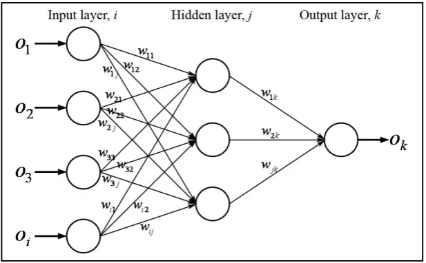
Figure 2.1 Simple Back Propagation Neural Network Architecture
Unlike other ANN architectures, BPNN learns by calculating the errors of the output layer to find the errors in the hidden layers. This makes BPNN highly suitable for problems in which no relationship is established between the output and the inputs. Due to its high rate of elasticity and learning abilities, it has been successfully applied in wide assortment of applications (Nawi at al., 2013). The main objective of the learning process is to minimize the difference between the actual output Ok and the desired output tk by adjusting the weights w* in the network optimally. The Error function is defined as (Gong, 2009);
21
2 1
n
k
k
k O
t
E (2.5)
where;
n : number of output nodes in output layer tk : desired output of the kth output unit Ok : network output of the kth output unit
11
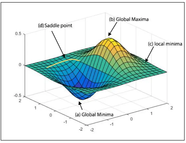
Figure 2.2 Schematic error functions for a single parameter w with stationary points
For networks with more than one layer, the error function is a non-linear function of weights and may have several minimum, which satisfies the following Equation and a 3D visualization is given in Figure 2.2:
E(w)0 (2.6)
Where E(w)denotes the gradient of E with respect to weights in Equation
2.6. In the Figure 2.2, the point at which the value of the error function is smallest is called the global minima at point (a) while all other minima are called local minima. There may also be other points, which satisfy the conditions in Equation (2.6) for instance global maxima at point (b) and saddle point at (c). Error is calculated by comparing the network output with the desired output by using Equation (2.6). The error signal E is propagated backwards through the network and is used to adjust the weights. This process continues until the maximum epoch or the target error is achieved by the network (Rehman and Nawi, 2011).
12
Ransing, 2006; Kolen and Pollack, 1990; Lahmiri, 2011; Rehman and Nawi, 2011; Zhang and Pu, 2011). An improper use of these parameters can lead to slow network convergence or even network fiasco. Therefore, several modifications have been suggested to stop network stagnancy and to speed-up the network convergence to global minima.
In 1989, Lari-Najafi indicated the use of large initial weights for increasing the learning rate of the BPNN network. Later, it was found that if the initial weight range is increased beyond the problem-dependant limit the network’s performance deteriorates (Lari-Najafi et al., 1989). In 1990, Kolen and Pollack proved the sensitivity of BPNN to initial weights and suggested the use of weights initialized with small random values (Kolen and Pollack, 1990). Therefore to make BPNN perform better, the selection of initial weights is vital and helps speed-up the network convergence to global minima (Abdul Hamid, 2012; Hyder et al., 2009).
Another BPNN parameter known as momentum coefficient is used to suppress oscillations in the trajectory by adding a fraction of the previous weight change (Fkirin et al., 2009). The addition of the momentum coefficient helps to smooth-out the descent path by avoiding extreme changes in the gradient due to local irregularities (Rehman and Nawi, 2011b; Sun et al., 2007). Hence, it is vital to suppress any oscillations that results from the changes in the error surface (Abdul Hamid, 2012). In the early 90’s, back-propagation with Fixed Momentum (BPFM) showed its prowess
13
iteration and oscillations are greatly suppressed with reduced error at the end of the final convergence. In 1994, Swanston, Bishop, & Mitchell proposed Simple Adaptive Momentum (SAM) for further improving the performance of BPNN (Swanston, Bishop, and Mitchell, 1994). In SAM, if the change in the weights is in the similar ‘direction’ then the momentum term is increased to accelerate the convergence
otherwise it is decreased. SAM has been found to have lower computational overheads than the conventional BPNN algorithm and it converged in considerably less iterations.
Later in 2008, Mitchell updated SAM by scaling the momentum after considering all the weights in each part of the Multi-layer Perceptrons (MLP). This technique is found helpful in improving convergence speed to the global minima (Mitchell, 2008). Shao & Zheng (2009) introduced a new Back Propagation momentum Algorithm (BPAM) with dynamic momentum coefficient. In BPAM, momentum coefficient was adjusted by combining the information about the current gradient and the weight change in the earlier phase. When the angle between the present negative gradient and the last weight change is less than 90°, the momentum coefficient is defined as a positive value to speed up learning. Otherwise, momentum is kept zero to guarantee the descent of the error gradient. The new algorithm was found better than previous algorithms by reducing oscillations in the trajectory (Shao and Zheng, 2009).
Besides momentum, another parameter that greatly affects the performance of BPNN is learning rate. A great level of debate has happened on the selection of learning rate since the inception of BPNN. In the earlier studies, the usual value of learning rate was kept constant. In 2001, Ye claimed that the constant learning is unable to answer the search for the optimal weights resulting in the blind search (Ye 2001). To avoid more trials and errors with the network training, Yu & Liu (2002) introduced back propagation and acceleration learning method (BPALM) with adaptive momentum and learning rate to answer the problem of fixed learning rate. Their method was tested on Parity problem, Optical Character Recognition (OCR) and 2-Spirals problem, the results were found to be far superior to any other previous improvements on BPNN.
14
learning rate can slow down the network convergence while too big learning rate can leads the network towards less optimal solutions. So, a learning rate should be selected very carefully to make the network perform efficiently.
Besides other factors effecting the performance of BPNN, an activation function represents an output node that is showing some synapses or nothing at all. Its basic function is to limit the amplitude of the output neuron. It generates an output value for a node in a predefined range as the closed unit interval [0,1] or alternatively [-1,1] which can be a linear or non-linear function (Nawi, Ransing, and Ransing, 2006; Rumelhart, Hinton, and Williams, 1986). In this study, the logistic sigmoid activation function is used which limits the amplitude of the output in the range of [0,1]. The activation function for the 𝑗𝑡ℎ node is given in the Equation (2.7);
j net ja c j
e
o
,1
1
(2.7)where,
l j
i ij i
j
net w o
a
1
, (2.8)
where,
j
o
: output of thej
thunit.i
o
: output of the thi unit.
ij
w
: weight of the link from unit i to unit j.j net
a
, : net input activation function for thej
th unit.j
: bias for thej
th unit.j
c
: gain of the activation function.15
learning rate, and momentum is further verified by Eom, Jung, and Sirisena (2003) when they automatically tuned gain parameter with the fuzzy logic. Nawi (2007) used the adaptive gain parameter in back propagation with conjugate gradient method. Abdul Hamid (2012) further extended the work by Nawi (2007) and proposed Adaptive gain parameter with adaptive momentum, and adaptive leaning rate. The proposed Back Propagation Gradient Descent with Adaptive gain, adaptive momentum, and adaptive learning (BPGD-AGAMAL) algorithm showed significant enhancement in the performance of BPNN on classification datasets.
Despite inheriting the most stable multi-layered architecture, BPNN algorithm is not suitable for dealing with the temporal datasets due to its static mapping routine(Güler, Übeyli, and Güler, 2005). In-order to use a temporal dataset on BPNN, all dimensions of the pattern vectors must be equal otherwise BPNN is rendered useless. However, an alternate approach known as Recurrent Neural Networks (RNN) is available which can map both temporal and spatial datasets and has short term memory to remember the past event thus highly influencing the output vectors (Gupta, McAvoy, and Phegley, 2000; Gupta and McAvoy, 2000; Übeyli, 2008) . The RNN are discussed in more detail in the next section.
2.3.2 Recurrent Neural Network (RNN)
Unlike the directed acyclic graph formation offered by Multilayer Perceptrons (MLP) trained with back propagation algorithm, Recurrent Neural Network (RNN) have diagraph formation. RNN possess the capability to store previous change made to any node in the network to be utilized in the future, thus making RNN flexible enough to to understand temporal datasets. Due to this learning elasticity, RNN have been deployed in several fields such as; simple sequence recognition, Turing machine learning, pattern recognition, forecasting, optimization, image processing, and language parsing etc. (Pearlmutter, 1995; Übeyli, 2008; Williams and Zipser, 1989; Gregor et al., 2014).
16
BPTT is that of unfolding (Boden, 2001), it is a training method for fully recurrent network which allows back propagation to train an unfolded feed-forward non-recurrent version of the original network. Once trained, the weights from any layer of the unfolded network are passed onto the recurrent network for temporal training (Gupta et al., 2000; Rumelhart et al., 1986). BPTT is quite inefficient in training long sequences (Gupta and McAvoy, 2000). Also, error deltas make a big change for each weight after they are folded back requiring a greater memory requirement. If, a larger time step is used, it diminishes the error effect called vanishing gradient thus making it totally infeasible to be applied on any dataset (Boden, 2001; Kolen and Pollack, 1990).
Unlike BPTT, Recurrent Back Propagation (RBP) bears a resemblance to the master or slave network of Lapedes and Farber, but it is architecturally simple (Pineda, 1987). In RBP network, the back propagation is protracted directly to train fully recurrent neural network. In this method, all the units are assumed to have continually evolving states (Gupta, et al., 2000). Pineda (1987) used RBP on temporal XOR with 200 patterns and found it to consume a lot of time. Also, BPTT and RBP are offline training methods and not suitable for long sequences due to more time consumption.
In 1989, Williams used online training of RNN in which the weights are updated while the network is running and the error is minimized at the end of each time step instead of at the end of the sequence. This method allows recurrent networks to learn tasks that require retention of information over time periods having fixed or indefinite duration (Williams and Zipser, 1989).
In partial recurrent neural network, recurrence in feed forward neural network is produced by feeding back the network outputs as additional input units (Jordan et al., 1991) or delayed hidden unit outputs (Elman, 1990). Also known as Simple Recurrent Neural Network (SRNN), Elman Recurrent Neural Network (ERNN) is one of the most popular form of partial RNN. An ERNN network is a relatively simple structure proposed by Elman to train a network whose connections are largely feed-forward with a careful selection of feedback context layer’s units to hidden units. The
17
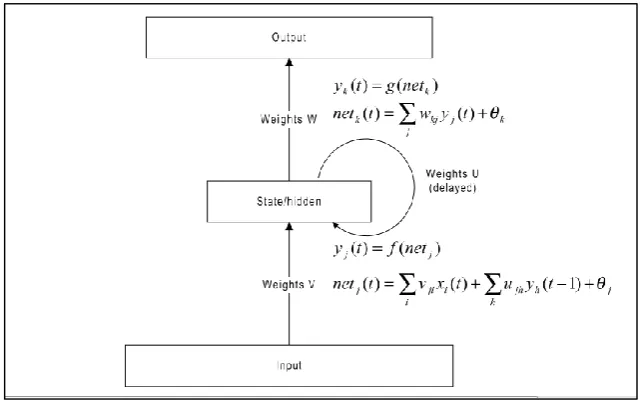
[image:40.595.158.480.181.381.2]Three layered ERNN is used in this research as given in the Figure 2.3. In ERNN, each layer has its own index variable: 𝑘 for output nodes, 𝑗 and h for hidden, and 𝑖 for input nodes. In a feed-forward network, the input vector 𝑥 is propagated through a weight layer 𝑉.
Figure 2.3 An Elman Recurrent Neural Network (Boden, 2001)
𝑛𝑒𝑡𝑗(𝑡) = ∑ 𝑥𝑛𝑖 𝑖(𝑡)𝑉𝑗𝑖+ 𝜃𝑗 (2.9)
Where, 𝑛 is the number of inputs, and 𝜃𝑗 is the bias. In an ERNN, the input
vector is spread in a similar manner like feed-forward networks propagate through a layer with some weights. But in RNN, the input vector is combined with the previous state activation through an additional recurrent weight layer, 𝑈;
𝑦𝑗(𝑡) = 𝑓(𝑛𝑒𝑡𝑗(𝑡)) (2.10)
𝑛𝑒𝑡𝑗(𝑡) = ∑ 𝑥𝑖𝑛 𝑖(𝑡)𝑉𝑗𝑖+ ∑ 𝑦𝑚𝑙 ℎ(𝑡 − 1)𝑈𝑗ℎ+ 𝜃𝑗 (2.11)
Where, 𝑓 is an output function and m is the number of states. The output of the network is achieved through the current state and the output weights, 𝑊;
18
𝑦𝑘(𝑡) = 𝑔(𝑛𝑒𝑡𝑘(𝑡)) (2.12)
𝑛𝑒𝑡𝑘(𝑡) = ∑ 𝑦𝑚𝑗 𝑗(𝑡 − 1)𝑊𝑘𝑗 + 𝜃𝑘 (2.13)
Where, 𝑔 is an output function, similar to 𝑓 and 𝑊𝑘𝑗 represents the weights from
hidden to output layer.
In the early 1990’s, ERNN has been found to have a sufficient generalization
capability and has successfully predicted the stock points in Tokyo stock exchange (Kamijo and Tanigawa, 1990). ERNN also takes advantage of the parallel hardware architecture, and it has shown faster capability to learn complex patterns such as natural language processing (Elman, 1991), and time series data classification (Husken and Stagge, 2003). In medical field, it is found beneficial in dynamic mapping of the electroencephalographic (EEG) signals classification with high accuracy during clinical trials (Güler et al., 2005).
Later, a similar ERNN technique was used for Doppler ultrasound signal classification using Lyapunov exponents and again high accuracy was achieved (Übeyli, 2008). Based on the optimization provided by ERNN, Xing (2015) has recently applied ERNN to solve real time price estimation problems in the power grid with great success (He et al., 2015). Despite all these achievements ERNN algorithms face the initial weight dilemma and gets stuck in local minima or slow convergence. In-order to avoid local minima and slow convergence in ANN, a second order derivative based Levenberg-Marquardt (LM) algorithm was introduced (Levenberg, 1944; Marquardt, 1963).
2.3.3 Levenberg-Marquardt (LM) Algorithm
19
of error surface is realistic, otherwise, the GN algorithm would be mostly divergent (Nawi et al., 2011).
Therefore an intermediary algorithm that utilizes the gradient descent and GN methods is introduced. The algorithm best known as Levenberg-Marquardt (LM) is more robust than the GN method, because in many cases it can converge even if the error surface is more complex than the quadratic situation (Levenberg, 1944; Marquardt, 1963). The elementary inkling of the Levenberg-Marquardt is that it shifts to the steepest descent algorithm, until the local curvature is proper to make a quadratic approximation; then it approximately becomes the Gauss–Newton algorithm, which can speed up the convergence significantly (Yu and Wilamowski, 2012). LM uses Hessian matrix for approximation of error surface. Assume the error function is:
𝐸(𝑡) =1
2∑ 𝑒𝑖 2(𝑡) 𝑁
𝑖=1 (2.14)
Where,
𝑒(𝑡): is the error, and
𝑁: is the number of vector elements, then;
∇𝐸(𝑡) = 𝐽𝑇(𝑡)𝑒(𝑡) (2.15)
∇2𝐸(𝑡) = 𝐽𝑇(𝑡)𝐽(𝑡) (2.16) Where,
∇𝐸(𝑡): is the gradient descent,
∇2𝐸(𝑡): is the Hessian matrix of E (t), and
𝐽 (𝑡): is Jacobian matrix
𝐽 (𝑡) =
[ 𝜕𝑣1(𝑡)
𝜕𝑡1
𝜕𝑣1(𝑡)
𝜕𝑡2 … . .
𝜕𝑣1(𝑡)
𝜕𝑡𝑛
𝜕𝑣2(𝑡)
𝜕𝑡1
𝜕𝑣2(𝑡)
𝜕𝑡2 … . .
𝜕𝑣2(𝑡)
𝜕𝑡𝑛
. . . 𝜕𝑣𝑛(𝑡)
𝜕𝑡1
𝜕𝑣𝑛(𝑡)
𝜕𝑡2 … . .
𝜕𝑣𝑛(𝑡)
𝜕𝑡𝑛 ]
(2.17)
20
∇𝑤 = −[𝐽𝑇(𝑡)𝐽(𝑡)]−1𝐽(𝑡)𝑒(𝑡) (2.18)
For the Levenberg-Marquardt algorithm as the variation of Gauss-Newton Method;
𝑤(𝑘 + 1) = 𝑤(𝑘) − [𝐽𝑇(𝑡)𝐽(𝑡) + 𝜇𝐼]−1𝐽(𝑡)𝑒(𝑡) (2.19)
Where 𝜇 > 0 and is a constant; 𝐼 is identity matrix. The algorithm will approach the Gauss- Newton which ought to deliver rapid convergence to global minima. Also, it should be kept in mind that when parameter λ is large, the Equation (2.19) approaches gradient descent (with learning rate 1/λ) while for a small λ, the algorithm approaches the Gauss- Newton method.
Although, LM possesses both the speed of the Gauss-Newton and the stability of the BPNN methods. But it has its limitations, one limitation is that the inverse of Hessian matrix needs to be calculated each time for weight update and this inversion may be repeated many times in a single epoch. Therefore, LM computation is efficient for small sized datasets. But for large datasets, such as image recognition datasets, LM may render itself useless as the Hessian inversion will be a CPU overhead. Another problem is that the Jacobian matrix has to be stored for computation, and its size is P × M × N, where P is the number of patterns, M is the number of outputs, and N is the number of weights. For large-sized training patterns, the memory cost for Jacobian matrix storage may be too huge to be practical. Also, for well-behaved functions and reasonable starting parameters, the LM tends to be a bit slower than the GN and has a high tendency towards convergence to local minima (Wilamowski et al., 2007).
21
In 2002, Ampazis and Perantonis presented two second-order algorithms for the training of feed-forward neural networks. The Levenberg Marquardt (LM) method used for nonlinear least squares problems incorporated an additional adaptive momentum term. The simulation results on large scale datasets show that their implementation models had better success rate than the conventional LM and other gradient descent methods (Ampazis and Perantonis, 2002). Later in 2005, Kermani implemented LM algorithm to determine the sensation of smell through the use of an electronic nose. Their research showed that the LM algorithm is a suitable choice for odor classification and it performs better than the old BP algorithm (Kermani et al., 2005).
Wilamowski et al. (2007) optimized the LM algorithm by calculating the Quasi-Hessian matrix and gradient vector directly, thus eliminating the need for storing the Jacobian matrix as it was replaced with a vector operation. The removal of Jacobian Matrix caused less memory overheads during simulations on large datasets. The simulation results found that this unconventional LM algorithm can perform better than the simple LM with less memory and CPU overheads (Wilamowski et al., 2007; H. Yu and Wilamowski, 2012). In recent years, several new LM modifications are proposed which will be discussed in more details in the Section 2.7.
Recently, metaheuristics belonging to the class of Swarm Intelligence have become quite popular due to their flexibility in providing derivative free solutions to complex problems. The Swarm Intelligent Metaheuristic algorithms are discussed in the next section.
2.4 Swarm Intelligent Metaheuristics
Swarm Intelligence is the collective behaviour of decentralized, self-organized systems, either natural or artificial. In 1989, Beny coined the term Swarm intelligence (Beni and Wang, 1989). Since then Swarm intelligence has become the basis of many nature inspired metaheuristic search algorithms. Meta means ‘to look beyond’ or ‘higher level’ and heuristic means ‘to find’ or ‘to discover by trial and error’. In short,
22
A metaheuristic optimization method is a heuristic strategy for probing the search space of an ultimately global optimum in a more or less intelligent way (Gilli and Winker, 2008). This is also known as a stochastic optimization. A stochastic optimization is grounded in the belief that a stochastic, high quality approximation of a global optimum obtained at the best effort will probably be more valuable than a deterministic, poor quality local minima provided by a classical method or no solution at all. Incrementally, it optimizes a problem by attempting to improve the candidate solution with respect to a given measure of quality defined by a fitness function. It first generates a candidate solution 𝑥𝑐𝑎𝑛𝑑𝑖𝑑𝑎𝑡𝑒and as long as the stopping criteria are not met, it checks its neighbours against the current solution (𝑆𝑒𝑙𝑒𝑐𝑡 𝑥𝑛𝑒𝑖𝑔ℎ𝑏𝑜𝑟∈ ℕ(𝑥𝑐𝑎𝑛𝑑𝑖𝑑𝑎𝑡𝑒)). The candidate solution is updated with its neighbour; if, it is
better (𝐼𝐹 𝑓(𝑥𝑛𝑒𝑖𝑔ℎ𝑏𝑜𝑟) < 𝑓(𝑥𝑐𝑎𝑛𝑑𝑖𝑑𝑎𝑡𝑒)𝑇𝐻𝐸𝑁 𝑥𝑐𝑎𝑛𝑑𝑖𝑑𝑎𝑡𝑒= 𝑥𝑐𝑎𝑛𝑑𝑖𝑑𝑎𝑡𝑒), such that the
global optimum at the end is 𝑥𝑜𝑝𝑡= 𝑥𝑐𝑎𝑛𝑑𝑖𝑑𝑎𝑡𝑒(Tang et al., 2012). As such,
metaheuristic optimization algorithms are often based on local search methods in which the solution space is not explored systematically or exhaustively, but rather a particular heuristic is characterized by the manner in which the exploration through the solution space is organized.
23
superior to that of many classical metaheuristics such as genetic algorithms (Goldberg, 1989) and particle swarm optimization (PSO) (Kennedy and Eberhart, 1995).
The main components of any metaheuristic search algorithm are exploration and exploitation. Exploration in metaheuristic algorithm is accomplished through the use of randomization provided by random walks to search much larger search space in the hope of finding more promising solutions. Exploration provides diversification which helps an algorithm to search globally and avoid local optima. On the other hand, exploitation process provides intensification in which new neighbourhood solutions are traversed locally to find a better solution than the already found optimal one (Neri and Tirronen, 2009; Yang et al., 2014). A review of the working process of the algorithms used in this research in-terms of exploration and exploitation are discussed in the remaining section.
Genetic Algorithm (GA) is a metaheuristic optimization algorithm that imitates the natural selection process while searching for the optimal solution (Holland, 1973; Goldberg, 1989). It is one of the oldest evolutionary search algorithm inspired by the natural evolution process, such as; mutation, selection, and crossover etc. In GA, number of solutions are considered as genomes or chromosomes. On the parent solutions, at each time-step the GA usually performs mutation and crossover to ultimately find the most optimal chromosome by exploring the solution. Meanwhile, the selection process helps in finding the fit individuals to transfer their information to the next generation in the evolutionary process; thus increasing the exploitation process in GA (Hansheng and Lishan, 1999).
Simulated Annealing (SA) is metaheuristic algorithm for finding an optimal solution for a stochastic problem. Proposed by Kirkpatrick, Gelett, and Vecchi (1983) and improved by Cerny (1985), this algorithm is inspired by the metallurgic process in which the metal is heated and cooled in a controlled manner to increase the durability of metal casting in the foundry (Černý 1985; Kirkpatrick et al., 1983). Only slow cooling process of metallurgy is implemented in SA with temperature as the main component for exploration and exploitation, so that SA will move from worse solutions to a final optimal one on the basis of probability of states with a minimum energy configuration (Bertsimas and Tsitsiklis, 1993).
24
based on the social behavior of bird flocking or fish schooling where each fish or bird is considered a particle (Kennedy and Eberhart, 1995). Like other evolutionary algorithms, these particles fly with a certain velocity to find the global best 𝑔𝑏𝑒𝑠𝑡
solution after traversing through several local best solutions in each iteration. It has been found highly efficient in solving several optimization problems such as; electromagnetics (Ciuprina et al., 2002), unsupervised robotic learning (Pugh, Martinoli, and Zhang, 2005), optimization of tile manufacturing process (Navalertporn and Afzulpurkar, 2011), and wireless sensor networks (Kulkarni and Venayagamoorthy, 2011) etc.
Since its origin in 2001, Harmony Search (HS) has been used extensively to solve many optimization problems such as vehicle routing (Geem, Lee, and Park, 2005), water distribution networks (Geem, 2006), numerical optimization (Karaboga and Akay, 2009), and University course time tabling (Al-Betar and Khader, 2012) etc. Proposed by Zong Woo Geem in 2001, HS algorithm is a metaheuristic algorithm based on the harmonic motion of sounds or melodies that human ears find pleasant to hear. This algorithm’s basic goal is to find an optimal solution just like a musician
produces a music note with perfect harmony (Geem et al., 2001). Harmony search utilizes three idealized rules based on the improvisation process of a musician, which are; harmony memory, pitch adjustment, and randomization (Yang, 2009). These rules are explained as follows;
a) HS memory is similar to the best fit individuals in the GA and the best harmony memory is carried over to the next harmony memory. Harmony memory is assigned a parameter known as 𝑟𝑎𝑐𝑐𝑒𝑝𝑡 ∈ [0,1], called acceptance rate.
Acceptance rate is neither kept too low nor too high, as it might leads to potentially less optimal solutions during exploitation process.
b) The second component of HS is the pitch adjustment rate controlled by pitch bandwidth 𝑏𝑟𝑎𝑛𝑔𝑒, and pitch adjusting rate 𝑟𝑝𝑎. In music pitch adjustment is
done to change frequencies but in HS it is used to generate change in the solution. Usually it is linearly adjusted to get;
REFERENCES
Ab Aziz, M. F., Shamsuddin, S. M. and Alwee, R. (2009). Enhancement of Particle Swarm Optimization in Elman Recurrent Network with Bounded Vmax Function. 3rd Asia International Conference on Modelling and Simulation, AMS 2009, 125–30.
Abdul Hamid, N. (2012). THE EFFECT OF ADAPTIVE PARAMETERS ON THE PERFORMANCE OF BACK PROPAGATION. Universiti Tun Hussein Onn Malaysia. Master Thesis.
Ackley, D. H. (1987). An Empirical Study of Bit Vector Function Optimization. Genetic algorithms and simulated annealing, vol. 1, 170–204.
Afrabandpey, H., Ghaffari, M., Mirzaei, A., & Safayani, M. (2014). A Novel Bat Algorithm Based on Chaos for Optimization Tasks. 2014 Iranian Conference on Intelligent Systems (ICIS), Iran, IEEE. 2–7.
Al-Betar, M. A., and Khader, A. H. (2012). A Harmony Search Algorithm for University Course Timetabling. Annals of Operations Research, vol. 194(1), 3– 31.
Alihodzic, A., and Tuba, M. (2014a). Improved Bat Algorithm Applied to Multilevel Image Thresholding. The Scientific World Journal, vol. 2014.
Alihodzic, A., and Tuba, M. (2014b). Improved Hybridized Bat Algorithm for Global Numerical Optimization. 2014 UKSim-AMSS 16th International Conference on Computer Modelling and Simulation, IEEE, 57–62.
Ampazis, N., and Perantonis, S. J. (2002). Two Highly Efficient Second-Order Algorithms for Training Feedforward Networks. IEEE Transactions on Neural Networks, vol. 13(5), 1064–74.
218
Battery Energy Storage for Micro-Grid Operation Management Using a New Improved Bat Algorithm. International Journal of Electrical Power & Energy Systems, vol. 56, 42–54.
Beni, G., and Wang, J. (1993). Swarm Intelligence in Cellular Robotic Systems. In Robots and Biological Systems: Towards a New Bionics? NATO ASI Series, vol. 102, 703–12.
Berman, S. M. (1971). Mathematical Statistics: An Introduction Based on the Normal Distribution. Intext Educational Publishers.
Bertsimas, D., and John, T. (1993). Simulated Annealing. Statistical Science vol. 8(1), 10–15.
Biswal, S., Barisal, A. K., Behera, A. and Prakash, T. (2013). Optimal Power Dispatch Using BAT Algorithm. 2013 International Conference on Energy Efficient Technologies for Sustainability, ICEETS 2013, 1018–23.
Blum, C. (2008). Hybrid Metaheuristics: An Emerging Approach to Optimization. Springer Berlin Heidelberg.
Blum, C., and Roli, A. (2003). Metaheuristics in Combinatorial Optimization: Overview and Conceptual Comparison. ACM Computing Surveys, vol. 35, 268– 308.
Boden, M. (2001). A Guide to Recurrent Neural Networks and Backpropagation. Electrical Engineering, (2), 1–10.
Bohachevsky Function (2015). www-optima.amp.i.kyoto-u.ac.jp/member/student/hedar/Hedar_files/TestGO_files/Page595.htm (July 4, 2015).
Brahim-Belhouari, S., and Bermak, A. (2004). Gaussian Process for Nonstationary Time Series Prediction. Computational Statistics & Data Analysis, vol. 47(4), 705–12.
Černý, V. (1985). Thermodynamical Approach to the Traveling Salesman Problem:
An Efficient Simulation Algorithm. Journal of Optimization Theory and Applications, vol. 45(1), 41–51.
219
Springer, vol. 6728, 28–37.
Ciuprina, G., Ioan, D. and Munteanu, I. (2002). Use of Intelligent-Particle Swarm Optimization in Electromagnetics. IEEE Transactions on Magnetics, vol. 38 (21), 1037–1040.
Collignan, A., Pailhes, J., and Sebastian, P. (2011). Design Optimization: Management of Large Solution Spaces and Optimization Algorithm Selection. In IMProVe, Venice.
Davis, R. A. 2007. Gaussian Processes. Encyclopedia of Environmetrics, vol. 3, 1–13.
Dwinell, W. (2007). AUC. http://matlabdatamining.blogspot.my/2007/06/roc-curves-and-auc.html (April 15, 2016).
Elman, J L. (1990). Finding Structure in Time. Cognitive science, vol. 14(2), 179–211.
Elman, J. L. (1991). Distributed Representations, Simple Recurrent Networks, and Grammatical Structure. Machine Learning, vol. 7(2-3), 195–225.
Eom, K., Jung, K. and Sirisena, H. (2003). Performance Improvement of Backpropagation Algorithm by Automatic Activation Function Gain Tuning Using Fuzzy Logic. Neurocomputing, vol. 50: 439–60.
Evett, I. W., and Spiehler, E. J. (1987). Rule Induction in Forensic Science. KBS in Government, 107–118.
Fawcett, T. (2004). ROC Graphs : Notes and Practical Considerations for Researchers. ReCALL, vol. 31(HPL-2003-4), 1–38.
Fawcett, T. (2006). An Introduction to ROC Analysis. Pattern Recognition Letters, vol. 27(2006), 861–74.
Fisher, R. A. (1936). The Use of Multiple Measurements in Taxonomic Problems. Annals of Eugenics, vol. 7(2), 179–88.
Fister Jr, I., Fister, I., and Brest, J. (2012). A Hybrid Artificial Bee Colony Algorithm for Graph 3-Coloring. Swarm and Evolutionary Computation, 66–74.
Fister, I., Fister, D., and Yang, X. S. (2013). A Hybrid Bat Algorithm. Elektrotehniski Vestnik/Electrotechnical Review, vol. 80, 1–7.
220
Fister, I., Fister Jr, I. and Zumer, J. (2012). Memetic Artificial Bee Colony Algorithm for Large-Scale Global Optimization. IEEE Congress on Evolutionary Computation (CEC),.
Fkirin, M. A., Badwai, S. M., and Mohamed, S. A. (2009). Change Detection Using Neural Network in Toshka Area. 2009 National Radio Science Conference.
Gandomi, A. H., and Yang, X. S. (2014). Chaotic Bat Algorithm. Journal of Computational Science, vol. 5, 224–32.
Geem, Z. W. , Kim, J. H. and Loganathan, G. V. (2001). A New Heuristic Optimization Algorithm: Harmony Search. Simulation, vol. 76, 60–68.
Geem, Z. W. (2006). Optimal Cost Design of Water Distribution Networks Using Harmony Search. Engineering Optimization, vol. 38(3), 259–77.
Geem, Z. W., Lee, K. S., and Park, Y. (2005). Application of Harmony Search to Vehicle Routing. American Journal of Applied Sciences, vol. 2(12), 1552–1557.
Ghosh, A., and Chakraborty, M. (2012). Hybrid Optimized Back Propagation Learning Algorithm For Multi-Layer Perceptron. International Journal of Computer Applications, vol. 57(December), 1–6.
Gilli, M., and Winker, P. (2008). A Review of Heuristic Optimization Methods in Econometrics. Swiss Finance Institute Research, 08–12.
Goldberg, D. E. (1989). Genetic Algorithms in Search, Optimization, and Machine Learning. Addison Wesley.
Gong, B. (2009). A Novel Learning Algorithm of Back-Propagation Neural Network. IITA International Conference on Control, Automation and Systems Engineering, (CASE 2009), 411–414.
Gonzalez, R. C., and Woods, R. E. (2008). Digital Image Processing. Prentice Hall.
Gregor, K., Danihelka, I., Graves, A., and Wierstra, D. (2014). DRAW: A Recurrent Neural Network For Image Generation.
Griewank, A. O. (1981). Generalized Descent for Global Optimization. Journal of Optimization Theory and Applications, vol. 34, 11–39.
221
Gupta, L., and McAvoy, M. (2000). Investigating the Prediction Capabilities of the Simple Recurrent Neural Network on Real Temporal Sequences. Pattern Recognition, vol. 33(12), 2075–2081.
Gupta, L., McAvoy, M. and Phegley, J. (2000). Classification of Temporal Sequences via Prediction Using the Simple Recurrent Neural Network. Pattern Recognition, vol. 33(10), 1759–1770.
Hagan, M. T., and Menhaj, M. B. (1994). Training Feedforward Networks with the Marquardt Algorithm. IEEE Transactions on Neural Networks, vol. 5(6), 989– 93.
Hale, D. (2006). Recursive Gaussian Filters. Proceedings of XVII IMEKO World Congress.
Han, J., and Kamber, M. (2006). Data Mining: Concepts and Techniques. Soft Computing, vol. 54.
Hansheng, L., and Lishan, K. (1999). Balance between Exploration and Exploitation in Genetic Search. Wuhan University Journal of Natural Sciences, vo. 4(1), 28– 32.
Hasançebi, O., and Carbas, S. (2014). Bat Inspired Algorithm for Discrete Size Optimization of Steel Frames. Advances in Engineering Software, vol. 67, 173– 85.
Hasançebi, O., Teke, T. and Pekcan, O. (2013). A Bat-Inspired Algorithm for Structural Optimization. Computers and Structures, vol. 128, 77–90.
He, X. (2015). A Recurrent Neural Network for Optimal Real-Time Price in Smart Grid. Neurocomputing, vol. 149, 608–612.
He, X. S., Ding, W. J., and Yang, X. S. (2013). Bat Algorithm Based on Simulated Annealing and Gaussian Perturbations. Neural Computing and Applications, vol. 25(2), 1–10.
Ho, Y., Bryson, A. and Baron, S. (1965). Differential Games and Optimal Pursuit-Evasion Strategies. IEEE Transactions on Automatic Control, vol. 10(4).
Holland, J. H. (1973). Genetic Algorithms and the Optimal Allocation of Trials. SIAM Journal on Computing, vol. 2(2), 88–105.
222
Classification. Neurocomputing, vol. 50, 223–35.
Hyder, M. M., Shahid, M. I., Kashem, M. A., and Islam, M. S. (2009). Initial Weight Determination of a MLP for Faster Convergence. Journal of Electronics and Computer Science, vol. 10.
Jacobs, R. A., Jordan, M. I., Nowlan, S. J., and Hinton, G. E. (1991). Adaptive Mixtures of Local Experts. Neural Computation, vol. 3(1), 79–87.
Jin, N., and Rahmat-Samii, Y. (2007). Advances in Particle Swarm Optimization for Antenna Designs: Real-Number, Binary, Single-Objective and Multiobjective Implementations. IEEE Transactions on Antennas and Propagation, vol. 55, 556–567.
Jong, D., and Alan, K. (1975). Analysis of the Behavior of a Class of Genetic Adaptive Systems. University of Michigan.
Jr, I. F., and Yang, X. S. (2013). A Hybrid Bat Algorithm. Elektrotehniski Vestnik/Electrotechnical Review, vol. 80(2), 1–7.
Kabir, W., Sakib, N. Chowdhury, S. M. R, and Alam, M. S. (2014). A Novel Adaptive Bat Algorithm to Control Explorations and Exploitations for Continuous Optimization Problems. International Journal of Computer Applications, vol. 94(13), 15–20.
Kamijo, K., and Tanigawa, T. (1990). Stock Price Pattern Recognition- A Recurrent Neural Network Approach. International Joint Conference on Neural Networks, 215–221.
Karaboga, D. (2005). An Idea Based on Honey Bee Swarm for Numerical Optimization. Technical Report TR06, Erciyes University (TR06).
Karaboga, D, and Akay, B. (2009). Artificial Bee Colony (ABC), Harmony Search and Bees Algorithms on Numerical Optimization. Proceedings of Innovative Production Machines and Systems Virtual Conference, IPROMS, 1–6.
Karaboga, D., and Basturk, B. (2008). On the Performance of Artificial Bee Colony (ABC) Algorithm. Applied Soft Computing Journal, vol. 8, 687–97.
Karaboga, D., and Akay, B. (2009). A Comparative Study of Artificial Bee Colony Algorithm. Applied Mathematics and Computation, vol. 214, 108–132.