Evaluation on flow discharge of grassed swale in lowland area

Evaluation on Flow Discharge of Grassed Swale

in Lowland Area

Nurhazirah Mustaffa1, Noor Aliza Ahmad1, *, and Mohd Adib Mohammad Razi1

1

Faculty of Civil and Environmental Engineering, Department of Water and Environmental Engineering, Universiti Tun Hussein Onn Malaysia, 86400 Parit Raja, Batu Pahat, Johor

Abstract. Grassed swale is an open vegetated channel designed

specifically in attenuating stormwater runoff to decrease the velocity, to reduce the peak flows, and minimize the causes of flood. Therefore, the fundamental of this study is to evaluate the flow discharge of swale in Universiti Tun Hussein Onn Malaysia (UTHM), which has flat land surface area. There are two sites of study were involved to assess the performance of swale as stormwater quantity control, named as swale 1 and swale 2. Data collection was conducted on 100 meters of length for each swale. The velocity of swale was measured thrice by using a current meter according to the six-tenths depth method, after a rainfall event. The discharge of drainage area in UTHM was determined by the Rational Method (Qpeak), and the discharge of swales (Qswale) was evaluated by the

Mean-Section Method. Manning’s roughness coefficient and the infiltration rate were also determined in order to describe the characteristics of swale, which contributing factors for the effectiveness of swale. The results shown that Qswale is greater than Qpeak at swale 1 and

swale 2, which according to the Second Edition of MSMA, the swales are efficient as stormwater quantity control in preventing flash flood at the campus area of UTHM.

1 Introduction

A rapid urbanization over the past few decades creates the need for construction of extensive storm drainage facilities [1]. Swales are one of the sustainable means to decrease the velocity, reduce the peak flows, and minimize the causes of flood, which applicable in many urban settings such as parking lots, roadways, commercial and light industrial facilities, and residential developments [2]. A grassed swale is a potential solution to transport stormwater from impervious surfaces by slowing down the flow and infiltrates into soils, and gives a significant improvement as a stormwater quantity and quality control over the traditional drainage ditch [3].

There are several factors that contributed to the ineffectiveness of urban drainage systems, such as topography, soil type, and substandard drainage design. In the case of Batu Pahat, Johor, some of the contributing factors include the lowland area where the land surface is flat and only 1 to 2 meters above sea level. Besides, the top soil is dominated by

*

soft clay and peat soils, which caused the low infiltration rate [4]. In the end of 2006, Batu Pahat has been hit by severe flood, which was called as “banjir termenung”. Universiti Tun Hussein Onn Malaysia (UTHM) was also affected by this flood where the old campus has been partially sunk in water. Even though UTHM has provided a detention pond, however, it is inefficiently functioned to reduce the peak flow rate as the elevation gabs is small between inflow and outflow, which caused back water from the main drain or river flows back into the drainage area [5].

Thus, the fundamental of this study is to find out whether grassed swale is one of the sustainable means to overcome flash flood. The performance of swale was assessed in terms of water quantity control by evaluating the flow discharge of swale. There are two sites of swales were involved in the campus area of UTHM, named as swale 1 and swale 2, which shown in Fig. 1. This study was carried out mainly referred to the Second Edition of Urban Stormwater Management Manual for Malaysia (MSMA).

Fig 1. Sites of swales in UTHM campus as swale 1 and swale 2.

2 Preliminary works

runoff coefficient (Cavg) for each site of swale, where C is the runoff coefficient of segment and A is the area of segment in hectares (ha).

∑

∑

=

A

CA

C

The lengths of swale for both swale 1 and swale 2 are 100 meters, and divided into three sections (Section A, Section B, and Section C). The distance from Section A to Section B and Section B to Section C is 50 meters respectively. Four meters of a tagging line were stringed transversely across each section of the swale. Three points of verticals or subsections were established on the tagging line, labeled as left, center, and right, to define the location for wading rod during the current metering work. These points were divided at the center point of tagging line and distributed the left and right points corresponding to the bottom width of swale where the most shallow flow depth of swale would occur after a rainfall event. This tagging line was also facilitated for the levelling work to define the surface profile of swale.

3 Flow discharge measurement

Discharge or flow rate is expressed as Q. The flow discharge conveyed in the grassed swale is determined under fully developed conditions. Swales should be designed to convey the peak flow of the 10-year storm without overtopping. The swales were studied by determining the discharge of drainage areas (Qpeak) in UTHM evaluated by the Rational

Method and the discharge of swales (Qswale) evaluated by the Mean-Section Method. Qswale

must be greater than Qpeak, which means the swales in UTHM are able to accommodate the

precipitation amount received by each swale.

3.1 Mean-Section Method

Mean-Section Method is used for calculating the discharge rate in the cross-sectional area of flow. To cope with the vertical distribution of velocity, measurements should be made at different depths in the water profile. This study has applied the depth of observation set at 0.6 of the total depth to measure the mean velocity, as the depth of water within the swale is less than 75 cm [6]. The equipment used to measure the velocity of swale in this study is a 1-D electromagnetic current meter (AEM1-D). The flow velocity of swale was measured three times at each vertical by waded the rod into the stream for several seconds to obtain the value as appeared on the display unit. During the measurement, the rod needs to be held in a vertical position, and the sensor of current meter must be opposition to the flow direction (facing the upper stream).

3.2 Rational Method

360

CiA

Q

=

General procedures for estimating peak flow using the Rational Method, first must select design ARI [10]. Average Recurrence Interval (ARI) is the average length of time between rain events that exceeds the same magnitude, volume, or duration [11]. In this study, swales are categorized as a minor system which has 10-year ARI. The average rainfall intensity (i) for this study is determined by the empirical equation to minimize error in estimating the rainfall intensity values from the IDF curves [7], expressed in Equation 3,

η

θ

λ

)

(

+

=

d

T

i

k

(3)

where the fitting constants of λ, κ, θ, and η were adopted from the rainfall station of Sembrong Dam (Site 1931003) as according to the Second Edition of MSMA in Table 2.B1. Meanwhile, T is the ARI and d is the storm duration.

4 Contributing factors

Besides evaluating the flow discharge of each swale, the roughness coefficient and infiltration rate of swale were also determined in order to describe the characteristics of swale, which contributing factors in the effectiveness of swale. Roughness coefficients represent the resistance to flood flows in channels and flood plains [12]. Equation 4 is used to determine the Manning’s roughness coefficient (n), where Q is the flow discharge, A is the cross-sectional area, R is the hydraulic radius, and S is the longitudinal slope. These hydraulic parameters can be obtained based on the plotted surface profile of each swale.

2 1 3 2

S

R

Q

A

n

=

The infiltration capacity of the soil indicates the maximum infiltration rate at a certain moment. The infiltration rate of each swale was determined as the campus of UTHM was claimed have high groundwater table and low infiltration rate. As noted by David [13], the swales are expected to have a decreasing capacity for infiltration storage, with the maximum infiltration rate decays asymptotically towards the saturated hydraulic conductivity of the soil. The occurrences of surface flow, storage, and eventual discharge within the swale were resulted once the rain exceeds the maximum infiltration rate. The infiltration test was carried out by using the double ring infiltrometer, which consists of two concentric stainless steel inner and outer rings. As according to ASTM D3385-03 standard test method, the rings were driven into the soil and partially filled with water. The drop of water level in the inner ring is measured over time to obtain the infiltration rate. This rate becomes constant when the saturated infiltration rate for the soil being measured has been reached. The infiltration rate (I) equation expressed as in Equation 5, where the sum of infiltration in millimeters divided by the accumulation of time in hours.

∑

∑

=

time on Infiltrati

5 Results and discussion

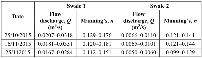
Data collection for swale 1 and swale 2 were carried out on three days, 25 October 2015, 16 November 2015, and 25 November 2015. The bottom widths at each section of swale are constant values, meanwhile the top widths are varied in line with the flow depth. The measurement of flow depth and velocity has found that the average flow depths for swale 1 (0.195 m – 0.390 m) are higher than swale 2 (0.120 m – 0.236 m). As well as the mean velocities of swale, swale 1 (0.088 m/s – 0.094 m/s) has the higher ranges of velocities than swale 2 (0.065 m/s – 0.078 m/s). The measurements of flow discharge and roughness coefficient were evaluated for each section of swale on the certain days, where the results are shown in Table 1.

Table 1. The flow discharges and roughness coefficients of both swales on three days.

Date

Swale 1 Swale 2

Flow discharge, Q

(m3/s)

Manning’s, n

Flow discharge, Q

(m3/s)

Manning’s, n

25/10/2015 0.0207–0.0318 0.129–0.176 0.0066–0.0110 0.121–0.141 16/11/2015 0.0181–0.0351 0.120–0.181 0.0065–0.0101 0.121–0.144 25/112015 0.0167–0.0284 0.112–0.151 0.0050–0.0060 0.099–0.129

From previous study by Ali et al. [14] have compared the surface roughness of swale between a gravel bed and smooth bed, where the gravel bed has a slightly higher coefficient than the smooth bed. It shows that the rough the surface, the higher the coefficient will occur. However, the results on Table 1 have shown otherwise, where the values of Q were increased as the n values increased. In this case, previous study by Stagge [9] has claimed that at high-flow depths, water is not slowed by grass in the swale but allowing sedimentation and too high to undergo filtration. The results from Table 1 were also found similar to the previous study by Rhee et al. [15], where when the flow depth is greater than the grass height, the submergence will occur and the roughness started to increase as the velocity increased. These findings have explained why the flow discharges in this study did not decrease as the swale bed gets rougher.

As stated by Temple et al. [16], in case of large flows, thickness of the boundary zone by vegetative growth tends to be a minimum, thus the passing flow becomes negligible and the roughness coefficient tends to converge to a constant. This has seconded by Wu et al. [17], as the submergence starts to occur in the swale, the roughness coefficient tends to remain constant or rise. He also added that heights, types, and conditions of the vegetation are the factors that contribute to the changes in flow characteristics of the swale and its roughness coefficient. This can be concluded that the variations of roughness coefficients occurred at each section of swales as shown in Table 1 are due to the characteristics of grass growth. There is a possibility that there are differences in heights, types, and conditions of the grass in each section of swale even in a same swale. However, this study did not perform an evaluation on the characteristics of grass.

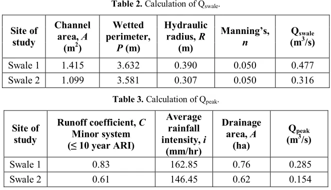
The calculation of flow discharge on swales (Qswale) and flow discharge on drainage

areas (Qpeak) are shown in Table 2 and Table 3 respectively. The channel areas in Table 2

were determined by applying the maximum flow depth of each swale. In evaluating the Qswale, the n values were according to Table 2.3 as in the Second Edition of MSMA, so that

Table 2. Calculation of Qswale.

Site of study

Channel area, A

(m2)

Wetted perimeter,

P (m)

Hydraulic radius, R

(m)

Manning’s,

n (mQswale3/s)

Swale 1 1.415 3.632 0.390 0.050 0.477

Swale 2 1.099 3.581 0.307 0.050 0.316

Table 3. Calculation of Qpeak.

Site of study

Runoff coefficient, C Minor system (≤ 10 year ARI)

Average rainfall intensity, i

(mm/hr)

Drainage area, A

(ha)

Qpeak

(m3/s)

Swale 1 0.83 162.85 0.76 0.285

Swale 2 0.61 146.45 0.62 0.154

The Qpeak in Table 3 was evaluated by using the Equation 2. Based on Table 2 and Table

3, the comparisons between Qswale and Qpeak can be made. The results shown that Qswale is

greater than Qpeak at swale 1 and swale 2, which according to the Second Edition of MSMA,

the swales are efficient as stormwater quantity control in preventing flash flood. The capability of swales at the campus area of UTHM in collecting and conveying the stormwater runoff are in the range of 48.7% – 59.7%. In terms of reducing the flow discharge, previous studies have found significant results of the effectiveness of swale. Stagge [9] has compared to the direct runoff and found that the swales reduced the peak flow by an average 50% - 53%. Based on flow attenuation for swale surface, Ainan et al. [18] have found the percentage reduction of peak flow in the range of 28.9% - 55.9%. In field studies by Wu et al. [19] and supported by swale hydrologic models [20, 21] have noted a percentage reduction of peak flows in the range of 10% - 20%. This percentage reduction of peak flow has proven the swale is capable in controlling the stormwater quantity.

Table 4. Summary of swale characteristics.

Criteria Site of study Swale 1 Swale 2

Drainage area, A (ha) 0.76 0.62

Channel length, L (m) 100 100

Longitudinal slope, So (m/m) 0.001 0.001

Channel area, A (m2) 1.415 1.099

Side slope, z 1.7 2.3

Maximum flow depth, y (m) 0.63 0.47

Infiltration rate, I (mm/hr) 21.14 4.67

Time of concentration, tc (min) 18.9 22.8

Percentage of impervious area (%) 77.6 38.7

Hydrologic soil group (HSG) is expressed in terms of four groups (A, B, C, and D) based on soil’s infiltration rate defined by Soil Conservation Service [22]. According to Table 4, swale 1 has the infiltration rate of 21.14 mm/hr, which categorized the soil in Group A. Group A soils have low runoff potential and high infiltration rates even when thoroughly wetted and consist chiefly of deep, well to excessively drained sands or gravels. Meanwhile, swale 2 has the infiltration rates of 4.67 mm/hr, which categorized the soil in Group B. Group B soils have moderate infiltration rates when thoroughly wetted and consist chiefly of moderately deep to deep, moderately well to well drained soils with moderately fine to moderately coarse textures. From the results, it shows that swale 2 has low rate of water transmission compared to swale 1.

6 Conclusions

This study has carried out flow discharge measurements of grassed swales in UTHM campus, which took place at swale 1 within the area of 0.76 ha and swale 2 within the area of 0.62 ha. Based on the analyses, swale 1 and swale 2 are an effective grassed swale in conveying stormwater runoff (Qswale >Qpeak). The swales are efficient in preventing flash

flood with the average rainfall intensity (i) of 146.45 mm/hr – 162.85 mm/hr. The results showed the flow discharges (Q) are increased by the increase of roughness coefficients (n). This can be concluded that the n values started to be constant or rise once the submergence occurs in the swale, where the flow depth is greater than the grass height. The heights, types, and conditions of the grass covers are the factors that contribute to the changes in flow characteristics of the swale and its roughness coefficient. In this study, both swales have 0.001 of longitudinal slope (So), however, differ in side slope (z) where swale 1 is 1.7 and swale 2 is 2.3. The n values at swale 2 have resulted slightly less than the n values at swale 1. This has shown that the channel irregularity of swales also may have contributed to the variations of n. This study can be extended to determine other contributing factors to the variations of flow discharges such as the types of vegetation or the rainfall intensity.

The authors would like acknowledgement the Ministry of Higher Education Malaysia and Research, Innovation, Commercialization, and Consultancy Management Office (ORICC) of Universiti Tun Hussein Onn Malaysia (UTHM) for financially under FRGS Fund (Vot 1414) for supporting this study.

References

[1] T.A. Saybet, Storm Water Management, Wiley, John & Sons, 179-191, (2006)

[2] City of Indianapolis, Stormwater Design and Specification Manual, Chapter 4.7 Swales, 104-112, Retrieved on September 16, 2016 from http:www.cityoffortwayne.org/utilities/images/stories/designman/ 4.7%20swales.pdf (2009)

[3] D. Stevens,For Three Weeks I Owned the University of Illinois, Lulu.com, 135-136, (2011)

[4] L.A.Q. Tunji, A.A.A. Latiff, D. Tjanjanto and S. Akib, The Effectiveness of Groundwater Recharges Well to Mitigate Flood, Int. J. of the Physical Sciences, 6 (1), 8-14, (2011)

[6] M.A. Khan, K. Mahmood and G.V. Skogerboe, Current Meter Discharge Measurements for Steady and Unsteady Flow Conditions in Irrigation Channels, Report No. T-7, Int. Irrigation Management Institute, Pakistan, (1997)

[7] Dept. of Irrigation and Drainage Malaysia (DID), Urban Stormwater Management Manual for Malaysia Second Edition, Government of Malaysia, (2012)

[8] A. Goyen, B.C. Phillips and S. Pathirajas, Urban Rational Method Review, Australia Rainfall and Runoff Revision Project 13, Engineers Australia, Canberra, (2014)

[9] J.H. Stagge, Field Evaluation of Hydrologic and Water Quality Benefits of Grass Swales for Managing Highway Runoff, Thesis of Master of Science, Faculty of Graduate School, University of Maryland, College Park, (2006)

[10] Dept. of Irrigation and Drainage Malaysia (DID), Urban Stormwater Management Manual for Malaysia, Government of Malaysia, (2000)

[11] V.T. Chow, Handbook of Applied Hydrology, McGraw-Hill Book, New York, (1964) [12] G.J. Jr. Arcement and V.R. Schneider, Guide for Selecting Manning's Roughness

Coefficients for Natural Channels and Flood Plains, U.S. Geological Survey Water Supply Paper 2339, United States Government Printing Office, Washington, (1989) [13] A.P. Davis, Field Performance Of Bioretention: Hydrology Impacts, J. Hydrologic

Engineering, ASCE, 13 (2), 90-95, (2011)

[14] Z.M. Ali and N.A. Saib, Influence of Bed Roughness in Open Channel, Proc. of Int. Seminar on Application of Science Mathematics, (2011)

[15] D.S. Rhee, H. Woo, B.A. Kwon and H.K. Ahn, Hydraulic Resistance of Some Selected Vegetation in Open Channel Flows, River. Res. Applic. 24, 673-687, (2008)

[16] D.M. Temple, K.M. Robinson, R.M. Ahring and A.G. Davis, Stability Design of Grass-lined Open Channels, Agricultural Handbook, 667, USDA: Washington, D.C., (1987)

[17] F. Wu, H.W. Shen and Y. Chou, Variations of Roughness Coefficients for Unsubmerged and Submerged Vegetation, J. of Hydra. Eng. ,125 (9), 239-245, (1999) [18] A. Ainan, N.A. Zakaria, A.A. Ghani, R. Abdullah, L.M. Sidek, M.F. Yusof and L.P.

Wong, Peak Flow Attenuation Using Ecological Swale and Dry Pond, Advances in Hydro-Science and Engineering, VI, (2003)

[19] J.S. Wu, C.J. Allan, W.L. Saunders and J.B. Evett, Characterization and Pollutant Loading Estimation for Highway Runoff, J. Envir. Eng., ASCE, 124(7), 584–592, (1998)

[20] A. Delectic, Performance of Grass Filters Used for Stormwater Treatment – A Field and Modeling Study, J. Hydrology, 317 (3-4), 168–182, (2006)

[21] D. Ackerman and E.D. Stein, Evaluating the Effectiveness of Best Management Practices Using Dynamic Modeling, J. Envir. Eng, ASCE 134 (8), 628–639, (2008) [22] R. Cronshey, R. H. McCuen, N. Miller, W. Rawls, S. Robbins, D. Woodward, J.