Embedded explicit two step Runge Kutta Nyström for solving special second order IVPs

http://dx.doi.org/10.12988/ams.2014.46403

Embedded Explicit Two-Step Runge-Kutta-Nystr¨

om

for Solving Special Second-Order IVPs

Department of Mathematics and Statistics,

Faculty of Science, Technology and Human Development Universiti Tun Hussein Onn Malaysia

86400 Batu Pahat, Johor, Malaysia

N. Senu, M. Suleiman and Z.A. Majid

Department of Mathematics and Institute for Mathematical Research Universiti Putra Malaysia, 43400 UPM Serdang

Selangor, Malaysia.

Copyright c2014 L. M. Ariffin, N. Senu, M. Suleiman and Z.A. Majid. This is an open access article distributed under the Creative Commons Attribution License, which permits unrestricted use, distribution, and reproduction in any medium, provided the original work is properly cited.

Abstract

A third-order three-stage explicit Two-step Runge-Kutta-Nystr¨om (TSRKN) method embedded into fourth-order three-stage TSRKN method is developed to solve special second-order initial value problems (IVPs) directly. The stability of the method is investigated. Numerical re-sults are obtained by solving a standard set of test problems, which then reduced to first-order system when solved using Runge-Kutta (RK) method and comparison are made with existing RK method with same order using variable step-size. The results clearly showed the advantage and the efficiency of the new method.

Mathematics Subject Classification: 65L05, 65L20

1

Introduction

Special second-order ordinary differential equations (ODE’s) is given by

y(_x) =_f(_{x, y}(_x)) (1)

with the initial conditions

y(_x0) =_{y0, y}(_x0) = _y0

where _y(_x)_f(_{x, y})∈_Rn_.

Equation (1) can be solved when using standard Runge-Kutta (RK) method provided that it has to be reduce to an equivalent first-order system of twice the dimension. However, Sharp and Fine [1], Dormand et al. [2] and El-Mikkawy and El-Desouky [3] shows that they manage to solve equation (1) directly and efficiently by using Runge-Kutta-Nystr¨om (RKN) method. In general, RK and RKN codes involving the embedded pairs of order _q(_p) is efficient when the method of order _q = _p+ 1 is used to obtain the numerical solutions of the problem where as the method of order _pis used to obtain the local trun-cation error. Unlike two-step RK method used in Jackiewicz and Verner [4], RK method for the numerical solution of (1) requires many evaluations of the function _fper step and hence is not as efficient as linear multistep methods, when the derivative evaluations are relatively expensive.

According to Senu et al. [5], when solving (1) numerically, the algebraic order of the method is essential where it is the main criterion to achieve high accuracy and to have lower stage of RKN method with maximal order in order to reduce the computational cost. Thus, in this paper we derive an embedded pair which is explicit and two-step in nature.

We consider the TSRKN method for the initial value problem (1) by Pa-ternoster [6] which was derived as an indirect method from the two-step RK method presented by Jackiewicz et al. [7], as follows

yi+2 = (1−θ)yi+1+θyi+h m

j=1

vjy

i+h

m

j=1

wjy

i+1+

h2 m

j=1

¯ vjf

xi+cjh, Yij

+ ¯_wjfxi+1+_{cjh, Yi}j₊₁ (2)

y_i+2 = (1−_θ)_yi+1+_θyi +_h

m

j=1

vjf

xi+cjh, Yij

+

wjf

xi+1+cjh, Yij+1

(3)

where

Yij+1 = yi+1+hcjy

i+1+h2

m

s=1

ajsf

xi+1+csh, Yis+1

Y_ij = _yi+_hcjyi+_h2

m

s=1

ajsf(xi+csh, Yis), j = 1, . . . m (4)

where _{θ, vj, wj,}¯_vj,w¯_{j, ajs}for _{j, s} = 1_{, . . . m} are the coefficients of the methods with _m is the number of stages for the method.

Alternatively TSRKN (2)and (3) can be written as

yi+2 = (1−θ)yi+1+θyi+h m

j=1

vjy

i+h

m

j=1

wjy

i+1+

h2 m

j=1

¯

vjkji + ¯wjkji+1 (5)

yi+2 = (1−θ)y

i+1+θy

i+h

m

j=1

vjkji +wjkji+1 (6)

where

k_ij = _f

xi+cjh, yi+hcjy

i+h2

m

s=1

ajskis

, j = 1_{, . . . m}

k_ij₊₁ = _f

xi+1+cjh, yi+1+hcjy

i+1+h2

m

s=1

ajsksi+1

, j= 1_{, . . . m.} (7)

Essentially, the methods derived should have the properties of zero stable and consistent. According to Paternoster [6], TSRKN is zero stable if −1_{< θ}≤1 and it is consistent ifm_j=1(_vj+_wj) = 1 +_θ. Fulfillment of these two properties implies that the method is convergent (see Watt [8] and Jackiewicz et al. [7]). Thus, we apply both properties into the derivation of our new method with θ= 0 that will guarantee zero stability of our method as proposed by Jackiewicz and Verner [4].

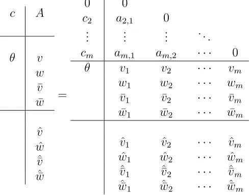
An embedded _q(_p) pair of TSRKN methods is based on the method (_{c, A, v, w,}¯_v,w¯) of order _q and the other TSRKN method (_{c, A,v,}ˆ _w,ˆ ˆ_v,¯ wˆ¯) of order _p(_{p < q}) which is similar with the embedded pair for one-step RKN derived by Senu et al. [5]. It can also be presented by the following Butcher array:

where _c = [_{c1, c2, . . . , cm}]T, _A = [_aij], _θ = 0, _v = [_{v1, v2, . . . , vm}]T, _w = [_{w1, w2, . . . , wm}]T, ¯_v = [¯_v1,v¯_{2, . . . ,v}¯_m]T, ¯_w= [ ¯_{w1, w}¯_{2, . . . ,w}¯_m]T, ˆ_v = [ˆ_{v1, v}ˆ_{2, . . . ,v}ˆ_m]T,

ˆ

w= [ ˆ_w1,wˆ_{2, . . . ,w}ˆ_m]T, ˆ¯_v =_vˆ¯_1,vˆ¯_{2, . . . ,}ˆ_v¯_m T and ˆ¯_w=wˆ¯1, wˆ¯2, . . . ,wˆ¯m T

Table 1: Embedded _m-stage 2-step explicit RKN method c A θ v w ¯ v ¯ w ˆ v ˆ w ˆ ¯ v ˆ¯ w = 0 0

c2 a2,1 0

..

. ... ... . . .

cm am,1 am,2 · · · 0 θ v1 v2 · · · vm

w1 w2 · · · wm

¯

v1 v¯2 · · · v¯m

¯

w1 w¯2 · · · w¯m

ˆ

v1 vˆ2 · · · vˆm

ˆ

w1 wˆ2 · · · wˆm

ˆ¯

v1 ˆv¯2 · · · ˆ¯vm

ˆ¯

w1 wˆ¯2 · · · wˆ¯m

2

Stability of the Method

In this section the linear stability of the TSRKN method will be discussed. By substituting

xi+1 =xi+h, yi+1=yi+hy

i+

h2 2 y

i, y

i+1 =y

i+hy

i

and apply the test equation _y = _f(_{x, y}) = −_λ2_y into TSRKN method (2) and (3), we obtain

yi+2 = yi+hy

i +

h2 2

−λ2yi

+_h

m

j=1

vjy

i +h

m

j=1

wj

y_i+_h−_λ2_yi+

h2 m j=1 ¯ vj

−λ2Yij

+ ¯_wj−_λ2_Yij₊₁ (8)

y_i+2 = _yi+_h−_λ2_yi+_h

m

j=1

vj

−λ2Y_ij+_wj−_λ2_Yij₊₁ (9)

where

Yij+1 = yi+hy

i+

h2 2

−λ2yi

+_hcjyi+_h−_λ2_yi+ h2 m s=1 ajs

−λ2Y_is₊₁ (10)

Yij = yi+hy

icj+h2

m

s=1

ajs

−λ2Yis

Multiply equation (9) by _h gives

hy_i+2 =_hyi+_h2−_λ2_yi+_h2

m

j=1

vj

−λ2Y_ij+_wj−_λ2_Yij_+1. (12)

The application of the test equation to equation (10) and (11) yields the re-cursion Y_i and Y_i+1 respectively.

Y_i =N−1_yie+_hyicandY_i+1=N−1_yie+eH₂ +c_H+_hyi(e+c)_. Elimination of the auxiliary vectors Y_i and Y_i+1 in equations (8) and (9) yields

yi+2 = yi

1 + H

2 +Hwe+H¯vN

−1_e+wN¯ −1_e+ H

2wN¯

−1_e+HwN¯ −1_c+

hy_i1 +ve+we+_HvN¯ −1c+wN¯ −1e+wN¯ −1c (13) hyi+2 = yi

H+_HvN−1e+_HwN−1e+H

2

2 wN

−1_e+H2_wN−1_c

+

hyi

1 +_HvN−1c+ _HwN−1e+ _HwN−1c (14)

with v= (_{v1, v2, . . ., vm})_, w= (_{w1, w2, . . ., wm})_, v¯= (¯_v1,v¯_{2, . . .,v}¯_m) andw¯ = ( ¯_w1,w¯_{2, . . .,w}¯_m) _.

The resulting recursion is Zi+2 =D(H)Zi with Zi+2 =

yi+2, hy

i+2

_T

and _Zi =_{yi, hyi}T

D(_H) =

A(_H) _B(_H) A(_H) _B(_H)

with

A(_H) = 1 + H

2 +Hwe+H¯vN

−1_e+wN¯ −1_e+H

2wN¯

−1_e+HwN¯ −1_c

B(_H) = 1 +ve+we+_H¯vN−1c+wN¯ −1e+wN¯ −1c

A(_H) = _H+_HvN−1e+_HwN−1e+H

2

2 wN

−1_e+H2_wN−1_c

B(_H) = 1 +_HvN−1c+ _HwN−1e+ _HwN−1c

whereN=_I−_{HA, H} =−(_λh)2_,c= (c_{1, . . . ,} c_s)T_, e= (1_{, . . . ,} 1)T with D(_H) is the stability matrix for the TSRKN methods above. The character-istic equation of _D can be written as

ξ2−trace(_D)_ξ+ det(_D) = 0 (15)

which is the stability polynomial of the TSRKN method.

Definition 2.1 (Absolute stability interval) An interval (−_Ha,0) is called the interval of absolute stability of the method (2) and (3) if for all _H ∈

3

Construction of the Method

The ETSRKN4(3) parameters must satisfy the following algebraic conditions as given in Ariffin et al. [9]. These order conditions was obtained in a more elementary way using the Taylor series expansion as proposed by Williamson [10]. Different approach was done by Jackiewicz et al. [7] where they used the theory of Hairer and Wanner [11] in order to derive the TSRK order conditions up to fourth-order. Here are the order conditions for TSRKN methods:

Order conditions for_y:

order 1 :

vi+wi = 1 (16)

order 2 :

wi+ ¯vi+ ¯wi =

3

2 (17)

order 3 :

¯

wi+civ¯i =

4 3,

¯

wi+ci(¯vi+ ¯wi) =

4

3 (18)

order 4 :

1 2

¯

wi+c2i¯vi =

2 3, 1 2 ¯

wi+ 2aijv¯i =

2

3, (19)

1 2

¯

wi+c2i(¯vi+ ¯wi) + 2ciw¯i=

2 3,

¯

wi+c2iv¯i+ciw¯i =

4

3. (20) Order conditions for_y

order 1 :

vi+wi = 1 (21)

order 2 :

wi+ci(vi+wi) = 2,

wi+civi = 2 (22)

order 3 :

1 2

wi+c2ivi =

4 3,

1 2

wi+ 2aijvi =

4

3, (23)

1 2

wi +c2i(vi+wi) + 2ciwi =

4 3,

wi+c2ivi+ciwi =

8

3 (24)

order 4 :

1 2

wi+ 2aijcivi = 2,

1 6

wi+c3ivi =

2

3, (25)

aijciwi = 0,

1 6

wi+c3i(vi+wi) + 3ciwi+ 3c2iwi =

2

1 2

wi+ciwi+ci2wi+c3ivi = 2,

1 2

wi+ciwi+ 2aijcivi = 2, (27)

1 2

wi+ciwi+c3ivi = 2,

aijcjvi =

2

3 (28)

Paternoster [12] gives the following definition:

Definition 3.1 An _m-stage TSRKN method is said to satisfy the following simplifying conditions if its parameters satisfy

m

j=1

aijckj−2 = ck

i

k(_k−1), i= 1, . . . , m, k= 1, . . . , q. (29)

Equation (29) allow the reduction of order conditions in the theory of TSRKN methods.

For the fourth-order method, solving simultaneously the equations (16)– (28) together with simplifying assumption (29). It involved 20 equations with 17 parameters and by setting _{c2, c3} and ¯_v3 as free parameters, the following solution of three-parameter family is obtained:

a21 = 1

2c

2

2, a31 = (c 2

2c3−4c2c3+ 2c2 −2c3+ 2c23)c3

2_c2(_c2 −2) , a32 = −c3(−c2c3+c2+c

2 3−c3)

c2(c2−2) , v1 =−

(−2_c3 + 3_c2c3−2_c2+ 4)

3_c2c3 ,

v2 = _{3(−1 +}2(c3−2)

c2)c2(c3−c2), v3 =−

2(_c2−2)

3_c3(−_c2c3+_c2+_c2₃−_c3), w1 = 2(−4c3+ 3c2c3+ 6−4c2)

3(−1 +_c2)(−1 +_c3) , w2 = 0, w3 = 0, ¯

v1 = −[6¯v3c33c2−6¯v3c33+ 12¯v3c23−6¯v3c23c22−6¯v3c23c2−6¯v3c3c2+

12¯_v3c3c2₂+ 11_c3c2₂−15_c3c2−6¯_v3c3+ 23_c2+ 6¯_v3c2−6¯_v3c2₂−15_c2₂]_/ [6_c2(−1 +_c2)(−1 +_c3)]_,

¯

v2 = −v¯3c3(−1 +c3)

c2(−1 +c2) ,w¯1 =

−4 + 4_c2−3¯_v3c3c2+ 3¯_v3c2₃

3(−1 +_c2) ,w¯2 = 0,w¯3 = 0. According to Dormand [2], the strategy to choose the free parameter is by minimizing the truncation error coefficients which are defined by

τ(p+1)

2 =

np+1

j=1

τj(p+1)

₂

andτ(p+1)

2 =

np+1

j=1

τj(p+1)

₂

for_ynand y_n respectively.

Letting_c2 = 5₆ gives||_τ(5)||₂in term of_c3. By using the minimize command in MAPLE, ||_τ(5)||₂ has a minimum value zero at _c3 = 3950₂₄₇₃. Since TSRKN is a two-step method, we may consider for the case _c3 ∈[0_,2]. Obtaining the value of_c3 gives||_τ(5)||₂ in terms of ¯_v3. Again, by using the minimize command

||τ(5)||2 has a minimum value zero at ¯v3 = 14579726695588_{37292647323125}. The above obtained

value of the free parameters gives ||_τ(5)||₂ = 2_.925926110901890175 ×10−2 and||_τ(5)||₂ = 4_.3167507760102019788×10−2. The stability interval of the fourth-order formula is approximately(-0.1805,0).

For the third-order method, using the same values for _aij and _ci obtained in the fourth-order method, solving the first four equations for_ynand the first seven equations for_yn simultaneously, the following solution of four-parameter is obtained:

¯

v1 = −1₅− 3348359_6115729v¯3,v¯2 =−24₅ + 42005880_6115729 ¯v3,

ˆ ¯

v2 = −35−6ˆv¯1+₂₄₇₃8862ˆv¯3+ 268639500_6115729 vˆ3,

ˆ

w1 = 6− 44773250_6115729 ˆv3,wˆ2 = 0,wˆ3 = 0,

ˆ¯

w2 = −4740₂₂₆₇wˆ¯1+144570₂₂₆₇ +23700₂₂₆₇ vˆ¯1− 23700₂₄₇₃ ˆ¯v3−468075000_6115729 vˆ3,

ˆ¯

w3 = 2473₂₂₆₇wˆ¯1− 150853₄₅₃₄ − 12365₂₂₆₇ vˆ¯1+ 5ˆv¯3+ 98750₂₄₇₃ ˆv3.

Using the minimize error approach; we obtain the value for all param-eters. By minimizing ||¯_τ(4)||₂, we obtain the minimum value zero at ˆ_v3 = 1_.0672840388671126404. However, we choose ˆ_v3 = 103₁₀₀ and it gives ||_τ¯(4)||₂ = 3_.6354254266897047443×10−2. Letting ˆ_v¯₁ = 3₂ and ˆ¯_w1 =−38221103_25000000, we obtain the value of ˆ¯_v3 with||_τ¯(4)||₂ = 1_.8965491105519564054×10−2. The coefficients in Table 2 are generated using MAPLE where the significant digits is set to 20 by the command Digits.

4

Problems Tested

Below are some of the problems tested:

Problem 1 (Homogeneous) d2y(_x)

dx2 =−64y(x), y(0) = 1, y

_{(0) =−2.}

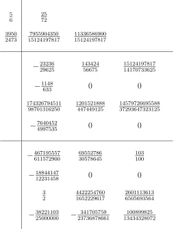
Table 2: Coefficients for ETSRKN4(3) method represented by Butcher array 0

5

6 2572

3950

2473 151241978177955904350 1133658690015124197817

−23236

29625 14342456675 1512419781714170733625

−1148

633 0 0

174326794511

98701316250 1201521888447449125 1457972669558837293647323125

−7640452

4997535 0 0

−467195557

611572900 6955278630578645 103100

−18844147

12231458 0 0

3

2 44222547601652229617 26011136136505693564

−38221103

The first order system: The new variable are _y1 =_y and _y2 =_y.

y1 =y2, y2 =−64y1, y1(0) = 1, y2(0) =−2, 0≤x≤50.

Exact solutions are _y1(_x) = −1_/4 sin(8_x) + cos(8_x)_{, y2}(_x) = −2 cos(8_x) − 8 sin(8_x)_.

Problem 2 (Inhomogeneous)

d2y(_x) dx2 =−v

2_{y(x) + (v}2_{−1) sin(x), y(0) = 1, y}

(0) =_v+ 1_{, x}≥0_, where _v 1_,0≤_x≤50_.

Exact solution is _y(_x) = cos(_vx) + sin(_vx) + sin(_x)_.Numerical result is for the case _v = 10_.

Source: van der Houwen and Sommeijer [13] The first order system:

y₁ =_{y2, y2}=−100_y1+ 99 sin(_x)_{, y1}(0) = 1_{, y2}(0) = 11_, 0≤_x≤50_. Exact solutions are_y1(_x) = cos(10_x)+sin(10_x)+sin(_x)_{, y2}(_x) =−10 sin(10_x)+ 10 cos(10_x) + cos(_x)_.

Problem 3

d2y1(x)

dx2 +y1(x) = 0.001 cos(x), y1(0) = 1, y

1(0) = 0

d2y2(x)

dx2 +y2(x) = 0.001 sin(x), y2(0) = 0, y

2(0) = 0.9995, 0≤x≤1000

Exact solutions are_y1(_x) = cos(_x)+0_.0005_xsin(_x)_{, y2}(_x) = sin(_x)−0_.0005_xcos(_x) Source: Stiefel and Bettis [14].

The first order system:

y₁ = _{y2, y2} =−_y1 + 0_.001 cos(_x)_{, y1}(0) = 1_{, y2}(0) = 0_,

y₃ = _{y4, y4} =−_y3 + 0_.001 sin(_x)_{, y3}(0) = 0_{, y4}(0) = 0_.9995_,0≤_x≤1000_. Exact solutions are

y1(x) = cos(x) + 0.0005xsin(x), y2(x) =−sin(x) + 0.0005xcos(x) + 0.0005 sin(x),

y1 = −y1

(

y21+y22)3

, y1(0) = 1, y1(0) = 0,

y2 = −y2

(

y21+y22)3

, y2(0) = 0, y2(0) = 1, 0≤x≤15π.

Exact solutions are _y1(_x) = cos(_x)_{, y2}(_x) = sin(_x). Source: Dormand et al. [2].

The first order system:

y₁ = _{y2, y2} =− y1 y21+y32

₃, y1(0) = 1, y2(0) = 0,

y₃ = _{y4, y4} =− y3 y21+y32

₃, y1(0) = 0, y2(0) = 1,0≤x≤15π.

Exact solutions are _y1(_x) = cos(_x)_{, y2}(_x) = −sin(_x)_{, y3}(_x) = sin(_x)_{, y4}(_x) = cos(_x)_.

Problem 5

d2y(_x)

dx2 =−y(x) +x, y(0) = 1, y

(0) = 2_,0≤_x≤500_.

Exact solution _y(_x) = sin(_x) + cos(_x) +_x. Source: Allen and Wing [15].

The first order system:

y1 =y2, y2 =−y1+x, y1(0) = 1, y2(0) = 2,0≤x≤500.

Exact solutions are _y1(_x) = sin(_x) + cos(_x) +_{x, y2}(_x) = cos(_x)−sin(_x) + 1_.

Problem 6 (Inhomogeneous System)

d2y1(x)

dx2 = −v

2_y

1(x) +v2f(x) +f(x), y1(0) =a+f(0), y1(0) =f

(0)_,

d2y2(x)

dx2 = −v

2_y

2(x) +v2f(x) +f(x), y2(0) =f(0), y2(0) =va+f

(0)_,0≤_x≤100_.

Source: Lambert and Watson [16]. The first order system:

y1 = y2, y2 =−16y1+ 16e−10x+ 100e−10x, y1(0) = 1.1, y2(0) =−10,

y3 = y4, y4 =−16y3+ 16e−10x+ 100e−10x, y3(0) = 1, y2(0) =−9.6.

Exact solutions are_y1(_x) = 0_.1 cos(4_x)+_e−10x_{, y}

2(x) =−0.4 sin(4x)−10e−10x, y3(x) =

0_.1 sin(4_x) +_e−10x_{, y}

4(x) = 0.4 cos(4x)−10e−10x. Problem 7 (Nonlinear System)

d2y1(x)

dx2 = −4x

2_y

1− y2

y12+y22

, y1(t0) = 0, y1(x0) =−

π/2

d2y2(x)

dx2 = −4x

2_y

2+ y1

y12+y22

, y2(x0) = 1, y2(x0) = 0,

π/2≤_x≤50

Exact solutions are _y1(_x) = cos(_x2)_{, y2}(_t) = sin(_x2)_. Source: Sharp et al. [17].

The first order system:

y₁ = _{y2, y2}=−4_x2_y1− 2y3 y12+y23

, y1(0) = 0, y2(0) =−

√

2_π,

y₃ = _{y4, y2}=−4_x2_y3+ 2y1 y21+y23

, y1(0) = 1, y2(0) = 0.

Exact solutions are_y1(_x) = cos(_x2)_{, y2}(_x) = −2_xsin(_x2)_{, y3}(_x) = sin(_x2)_{, y4}(_x) = 2_xcos(_x2)_.

5

Implementation and Numerical Results

The set of test problems in section 4 is solved using the new method and the results are compared with the numerical results when the same set of test problems are reduced to first order system twice the dimension and solve using method by Fehlberg [18] and Butcher [19]. For the new method and the existing methods, the next step size is determined by

hnew = 0.4×

T OL 2×_{LT E}

p+1

×hold

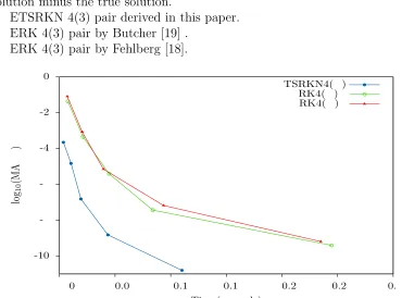
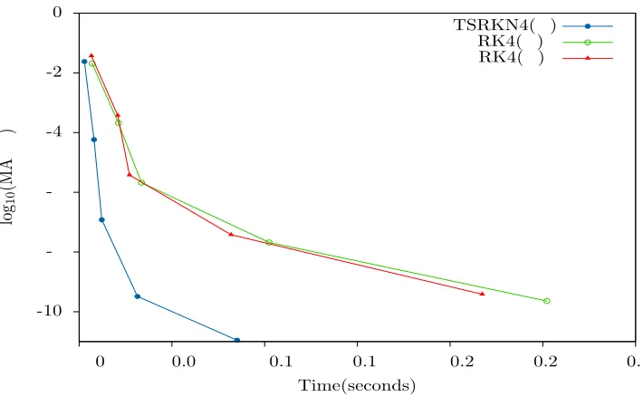
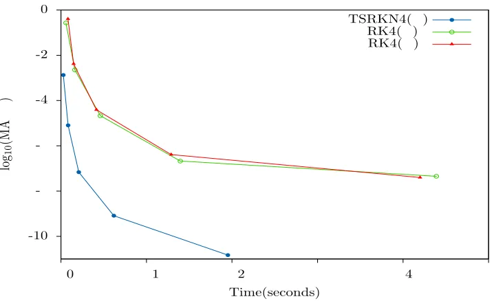
The numerical results are given in Figs. 1-7 and the notations used as follows:

MAXE – maximum global error (max_yn−_y(_xn)), that is the computed solution minus the true solution.

ETSRKN 4(3) pair derived in this paper. ERK 4(3) pair by Butcher [19] .

ERK 4(3) pair by Fehlberg [18].

RK4( ) RK4( ) TSRKN4( )

Time(seconds)

lo

g10

(MA

)

0. 0.2

0.2 0.1

0.1 0.0

0 0

-2

-4

--10

RK4( ) RK4( ) TSRKN4( )

Time(seconds)

lo

g10

(MA

)

0. 0.

0.4 0.

0.2 0.1

0 0

-2

-4

--10

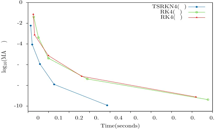
Figure 2: The efficiency curves of the ETSRKN4(3) method and its compar-isons for Problem 2 with _xend= 50

RK4( ) RK4( ) TSRKN4( )

Time(seconds)

lo

g10

(MA

)

0. 0. 0. 0. 0. 0.4 0.

0.2 0.1

0 0

-2

-4

--10

RK4( ) RK4( ) TSRKN4( )

Time(seconds)

lo

g10

(MA

)

0.1 0.0

0.0 0.04

0.02 0

0

-2

-4

--10

Figure 4: The efficiency curves of the ETSRKN4(3) method and its compar-isons for Problem 4 with _xend= 15_π

RK4( ) RK4( ) TSRKN4( )

Time(seconds)

lo

g10

(MA

)

0. 0.2

0.2 0.1

0.1 0.0

0 0

-2

-4

--10

RK4( ) RK4( ) TSRKN4( )

Time(seconds)

lo

g10

(MA

)

0.4 0.

0. 0.2 0.2 0.1

0.1 0.0

0 0

-2

-4

--10

Figure 6: The efficiency curves of the ETSRKN4(3) method and its compar-isons for Problem 6 with _xend= 100

RK4( ) RK4( ) TSRKN4( )

Time(seconds)

lo

g10

(MA

)

4 2

1 0

0

-2

-4

--10

6

Discussion and Conclusion

From Figures 1-7, we observed that ETSRKN4(3) is more efficient when com-pared to ERK4(3)B and ERK4(3)F in terms of computational time. This is due to the fact that when second-order problems is solve using method ERK4(3)B and ERK4(3)F, it has to be reduce to first-order system that is twice its dimension. In terms of global error, ETSRKN4(3) produced smaller error compared to ERK4(3)B and ERK4(3)F for all problems except for prob-lem 4 where ETSRKN4(3) global error is comparable with ERK4(3)B and ERK4(3)F. Thus we can conclude here that ETSRKN4(3) is more efficient than the existing technique where all the special second-order problems are solved directly whereby for other techniques, the problems need to reduce to first-order system of ODEs. Hence less time is needed to solve the same set of problems.

References

[1] P.W. Sharp and J.M. Fine, Some Nystr¨om pairs for the general second-order initial-value problem, Journal of Computational and Applied Math-ematics, 42 (1992), 279-291.

[2] J.R. Dormand, M.E.A. El-Mikkawy and P.J. Prince, Families of Runge-Kutta-Nystr¨om Formulae, IMA Journal of Numerical Analysis, 7(1987), 235-250.

[3] M.E.A. El-Mikkawy and R. El-Desouky, A new optimized non-FSAL em-bedded Runge-Kutta-Nystr¨om algorithm of orders 6 and 4 in six stages,

Applied Mathematics and Computation,145 (2003), 33-43.

[4] Z. Jackiewicz and J.H. Verner, Derivation and Implementation of Two-Step Runge-Kutta Pairs, Japan J. Indust. Appl. Math., 19 (2002), 227-248.

[5] N. Senu , M. Suleiman and F. Ismail, An embedded explicit Runge-Kutta-Nystr¨om method for solving oscillatory problems, Phys. Scr., 80 (2009), 015005 (7pp)

[7] Z. Jackiewicz,R. Renaut and A. Feldstein, Two-Step Runge-Kutta Meth-ods,SIAM J. Numer. Anal,28 (1991), 1165-1182.

[8] J.M. Watt, The asymptotic discretization error of a class of methods for solving ordinary differential equations, Proc. Cambridge Philos. Soc., 61

(1967), 461-472.

[9] L.M. Ariffin, N. Senu and M. Suleiman, A three-stage explicit two-step Runge-Kutta-Nystr¨om method for solving second-order ordinary differen-tial equations, National Symposium on Mathematical Sciences, AIP Conf. Proc. 1522, (2013), 323-329.

[10] R.A. Williamson Numerical Solution of Hyperbolic Partial Differential Equations, Ph.D. Thesis, Churchill College, Cambridge, (1984).

[11] E. Hairer and G. Wanner, Multistep-Multistage-Multiderivative Methods for Ordinary Differential Equations,Computing,11 (1973), 287-303. [12] B. Paternoster, Two Step Runge-Kutta-Nystr¨om Methods for Oscillatory

Problems Based on Mixed Polynomials, P.M.A. Sloot et. al. (Eds): ICCS 2003, LNCS 2658 (2003), 131-138.

[13] P.J. van der Houwen and B.P. Sommeijer, Explicit Runge-Kutta(-Nystrom) methods with reduced phase errors for computing oscillating solutions, SIAM J. Numer. Anal. 24 (1987), 595-617.

[14] E. Stiefel and D.G. Bettis, Stabilization of Cowell’s methods, Numerische Mathematik,13 (1969), 154-175.

[15] R.C. Allen Jr. and G.M. Wing, An invariant imbedding algorithm for the solution of inhomogeneous linear two-point boundary value problems,

Journal of Computational Physics,14 (1974), 40-58.

[16] J.D. Lambert and I.A. Watson, Symmetric multistep methods for periodic initial value problems, IMA Journal of Applied Mathematics, 18 (1976), 189-202.

[17] P.W. Sharp, J.M. Fine and K. Burrage, Two-stage and Three-stage Diag-onally Implicit Runge-Kutta-Nystr¨om methods of orders three and four,

IMA Journal of Numerical Analysis, 10 (1990), 489-504.

[18] E. Fehlberg, Classical Runge-Kutta fourth-order and lower order formulas with step size control and their application to Waermeleitungs problem,

[19] J.C. Butcher,The Numerical Analysis of Ordinary Differential Equations: Runge-Kutta and General Linear Methods, John Wiley & Sons, Great Britain, (1987).