Noise estimation by utilizing mean deviation of smooth region in noisy image

(1)

Performance Comparison Between Queueing Theoretical Optimality and Q-learning

Approach for Intersection Trafﬁc Signal Control

Pitipong Chanloha∗, Wipawee Usaha†, Jatuporn Chinrungrueng‡and Chaodit Aswakul§

∗_{Department of Electrical Engineering, Faculty of Engineering, Chulalongkorn University}

Patumwan, Bangkok, Thailand, 10330. Email: [email protected]

†_{School of Telecommunication Engineering, Institute of Engineering, Suranaree University of Technology}

Muang district, Nakhon Ratchasima, Thailand, 30000. Email: [email protected]

‡_{National Electronics and Computer Technology Center (NECTEC), Thailand Science Park, Klong Luang,}

Pathumthani, 12120 Thailand. Email: [email protected]

§_{Department of Electrical Engineering, Faculty of Engineering, Chulalongkorn University}

Patumwan, Bangkok, Thailand, 10330. Email: [email protected]

Abstract—This paper proposes the performance comparison for optimal traffic signal controls based on the following two frameworks: M/M/1 and D/D/1 queueing models, and Q-learning approach. Firstly, using the M/M/1 and D/D/1 models, the optimal split derivation has been obtained to minimise the mean waiting time of an intersection. Additionally, the Q-learning framework has been proposed in conjunction with the use of the macroscopic cell transmission model (CTM) to update the vehicle state dynamics upon Q-learning actions. The two approaches have been compared in terms of the network throughput and the average vehicle delay per completed trip in nine scenarios. The simulation results from the microscopic AIMSUN traffic simulator show that the Q-learning approach can greatly improve the intersection throughput and can sig-nificantly reduce the average vehicle delay per completed trip with the respective M/M/1 and D/D/1 approaches.

Keywords-Q-learning, queueing theory, cell transmission model (CTM).

I. INTRODUCTION

Due to the increase of traffic demands, the burden on the traffic control systems becomes a major concern. From the past history, the first sophisticated traffic control strategy has been manually operated by a policeman. The evolution of the control methodology for traffic signal grows rapidly. Fortunately, the growing emphasis on information systems and communication technologies is able to handle the traffic problem by using advanced traffic information and control systems. One of the most common goals of the researchers is to improve the efficiency of the traffic signal control by maximising the traffic throughput at an intersection.

Methods have been reported in the literature for control-ling traffic signals at an intersection. Due to the capacity limitation of urban area, it is therefore critical to improve the performance of traffic network. A classical method is to analyse an isolated traffic intersection in the steady-state by adopting the queueing theory for traffic signal control. Yu and Stubberud [1] are the first to address the traffic signal

proposes an adaptive control strategy for traffic signal control by modifying the green time until a queue vanishes within a finite time horizon. Mirchandani and Ning [3] develop and evaluate an adaptive signal control method based on queueing theory. Their proposed method is based on the in First-out (FIFO) queueing systems. The method trying to minimise the average vehicle delay by using minimal weight matching has been proposed by Wunderlich et. al [4]. The shortcoming of these analytical methods is that they cannot deal with abrupt changes of traffic patterns.

To cope with the dynamic changes, a flexible approach has been proposed to learn good traffic signal controls from experiences gained gradually by interacting directly with the environment. This approach, referred to as a reinforcement learning (RL), is a class of machine learning related to the ar-tificial intelligence [5]. RL is a class of unsupervised learning that has potentials to deal with traffic engineering problems [6]. Jacob and Abdulhai [7] addresses Q-learning which is an RL tool to deal with the highway traffic problems. For an isolated intersection control, [8], [9], [10], [11] consider Q-learning with different objective functions, whereas [12] investigates the green splits weighted by employing RL in order to minimise the number of vehicles in the system. Hong et. al [13] and Choy et. al [14] investigate the traffic signal control using a neural network which yields a high computational complexity and results in the impracticality in realistic scenarios. The literature above seek for an optimal traffic signal control for an isolated intersection. However, these RL approaches have been considered the individual movement of the vehicles in the microscopic level. Therefore, the computational burden becomes demanding.

(2)

state of the system. However, this paper differs from [15] in that we are interested in the trafﬁc signal control instead.

In addition, this paper compares the performance of Q-learning with the optimal split which has been derived for an isolated intersection with two conﬂicting ﬂows whose steady state dynamics are captured by two queueing models, i.e. M/M/1 and D/D/1. The comparative results have been reported from our AIMSUN platform.

The rest of this paper is organised as follows. Section II presents the optimal split formula for the trafﬁc queueing models. Section III formulates the Q-learning approach ex-plainable in two parts. Firstly, the state of the system uses CTM to update ﬂow dynamics. Secondly, the Q-learning algorithm is presented in Section IV. The simulation results are given in Section V and the conclusion is given in Section VI.

II. QUEUEINGTRAFFICMODEL

[image:2.612.316.552.70.203.2]

This section introduces a simplified queueing model with two buffers and single server which can be mapped into two conflicting flows in an isolated intersection.

Figure 1. Model for two conﬂicting ﬂows in an isolated intersection.

Fig. 1 illustrates an isolated intersection which serves two ﬂows from west to east and north to south. Fig. 1 can be converted into a basic queueing model with two buffers and a single server as shown in Fig. 2, where λp denotes the

trafﬁc arrival rate of the system for directionp= 1,2. Letμ

be the intersection service rate of the system. Letwpbe the

ratio of green time allocated to directionp(or its split) in a signal cycle. The objective here is to ﬁnd the optimal split

wp∗ that minimises the mean waiting time of the considered

[image:2.612.58.297.336.536.2]

intersection system.

Figure 2. Queueing model with two incoming requests.

A. Steady State Analysis

The steady-state derivation is based on an M/M/1 queue-ing model where the vehicle arrivals in each direction are assumed to be an independent Poisson process and, during their green time period, each vehicle is assumed to spend exponentially distributed travel time through the intersection. As illustrated in Fig. 1, an intersection has two individual conﬂicting ﬂows with mean arrival ratesλ1 andλ2,

respec-tively. Letμbe the saturation ﬂow rate, the ﬂow rate at which vehicles can pass through a signalised intersection in a stable moving queue [16]. Letρpbe the offered load in directionp

soρp= _wλ_pp_μforp= 1,2. To guarantee the stability condition

of the system, it is assumed that the intersection’s saturation ﬂow rate is greater than the total input ﬂow rate from all approaching directions. LetLdenote the total loss time value per signal cycle being normalised by the cycle period. Thus,

∀p

wp+L = 1. (1)

In the queueing steady state, the mean waiting timeTpin the

system for directionp can then be obtained as follows [17]

Tp = ₁₋ρp

ρp

= λp

wpμ−λp. (2)

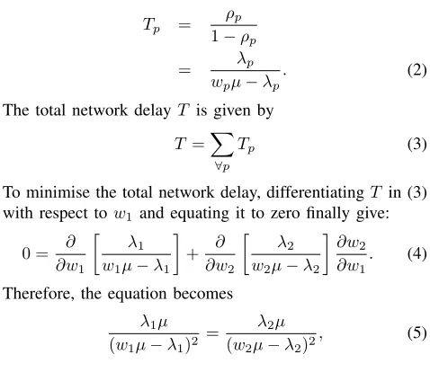
The total network delayT is given by

T =

∀p

Tp (3)

To minimise the total network delay, differentiatingT in (3) with respect tow1 and equating it to zero ﬁnally give:

0 = ∂

∂w1

λ1

w1μ−λ1

+ ∂

∂w2

λ2

w2μ−λ2

∂w2

∂w1. (4)

Therefore, the equation becomes

λ1μ (w1μ−λ1)2 =

λ2μ

[image:2.612.313.552.487.694.2]

(3)

where

∂w1

∂w1 +

∂w2

∂w1 +

∂L ∂w1 =

∂1

∂w1 (6)

∂w2

∂w1 = −1. (7)

The optimal split from M/M/1 modelw∗₁_,MM₁andw∗₂_,MM₁

can be expressed ﬁnally as

w∗₁_,MM₁ =

Λ (1−L) +λ1−λ2Λ

μ

(1 + Λ)

w∗₂_,MM₁ =

(1−L) +λ2Λ−λ1

μ

(1 + Λ) , (8)

whereΛ = λ1/λ2. This result from equation (8) represents

an optimal split weighted to each individual ﬂow.

In a realistic scenario, the arrival process and queueing service time may not be Poisson and exponential. Thus, in this paper, another model, D/D/1, has also been used, where the incoming stream of vehicles arrive at a ﬁxed deterministic rate and their service time through the intersection is assumed constant for every vehicle. The optimal split of D/D/1 model can be obtained similarly to the case of M/M/1 model and the ﬁnal result becomes

w∗₁_,DD₁ = Λ(1−L)

(1 + Λ)

w∗₂_,DD₁ = 1−L

(1 + Λ). (9)

III. Q-LEARNINGMODEL

A. State Space Deﬁnition

DefineSas the state space of the intersection system with two conflicting flows. Let s ∈ S ⊂Z2₊ be the state vector which represents the total number of vehicles waiting for the green light at the intersection. Letsp(t)be the state variable

which represents the number of vehicles in direction p at time instancetwherep= 1,2. Therefore, the state space S of all vehicle proﬁles in the system is given by

S:={s= [s1(t), s2(t)]}. (10)

B. Cell Transmission Model

CTM [18] is here employed to update the Q-learning state dynamics. CTM captures the effect of control actions decided by Q-learning on the ﬂow of vehicles in the system. The updating state depends on the green time allocated to each of approaching directions. The updating process of CTM can be summarised as follows.

1) Sending Capability: Letyp(t)be the number of

vehi-cles that can pass through the intersection in direction p at time stept:

yp(t) = min{sp(t), qp(t)}, (11)

whereqp(t)represents the maximum ﬂow rate at which

vehi-cles can ﬂow from their intersection upstream to downstream road segments along each directionpat time stept.

2) Receiving Capability:The receiving capability in CTM

normally depends on the maximum ﬂow rateqp(t)as

rp(t) = min{qp(t), εp(t)}, (12)

where εp(t)denotes the residual capacity in direction p at time stept.

C. Action Space Deﬁnition

In each interval, the agent must select whether it would remain in the current signal indication or change it. The decision is referred to as anaction. The action space, denoted byA, is the set of all possible actions which the trafﬁc signal controller of the considered intersection can take. Action

a ∈ A(s) refers to the action which the agent can take at state s.

D. Vehicle Delay

Vehicle delay is deﬁned as the number of vehicles that cannot pass through the intersection. The vehicle delay accumulated at time step tcan be expressed as

dp(t) =sp(t)−yp(t). (13)

Note that if the allocated green time can serve all trafﬁc in

sp(t), i.e.,sp(t) =yp(t), then there is no delay happening.

E. Reward Function

The aim of Q-learning here is to ﬁnd the optimal policy that minimises the total network delay, which can be ex-pressed in terms of the delaydp(t)at each time step tas:

Υ(t) =

∀p

dp(t)

=

∀p

(sp(t)−yp(t)). (14)

Note that qp(t)is affected by the action a, which speciﬁes

the direction that receives the green light as follows

qp(t) =

μ , a=p

0 , a=p. (15)

Equation (15) represents an action which allows the vehicles to pass through the intersection in direction pat time step t. The state dynamics of CTM can then be updated in according to the chosen action in each time step as

sp(t+ 1) =sp(t) +xp(t)−yp(t), (16) where xp(t) represents the newly incoming demands in

(4)

Table I

PSUEDO-CODE OFQ-LEARNINGALGORITHM[5]

1. InitialiseQ(s, a)arbitrarily (here, set to zeros). 2. Repeat (for each episode):

3. Initialisesto the state of empty roads 4. Repeat (for each time step of episode):

5. ChooseafromA(s)using policy derived fromQ

(e.g., we adopt the-greedy)

6. Take actiona, observeΥ, and the next CTM states as the result of the taken action

7. Update the action value function:

Q(s, a)←Q(s, a)+α[Υ +γminaQ(s, a)−Q(s, a)] 8. Update to the next CTM state:s←s;

9. until the end of simulation period.

IV. Q-LEARNINGALGORITHM

Table I depicts the standard Q-learning algorithm which is applied to solve the problem formulated as an MDP.

In Table I,Q(s, a)represents theaction valuefunction rep-resenting the average future reward expected to be incurred given that the action a has been taken at the state s [5]. According to the epsilon greedy policy, on the best apparent action will be selected with high probability of 1−, and the other actions will be tried out randomly with a small probability of. Therefore, the best apparent action orgreedy

action is exploited most of the time. And with probability

, the concept of exploration is to ensure that all of states are adequately visited. The parameter α is a small positive fraction, namely, the step-size parameter which inﬂuences the learning rate. Step-size parameter determines how much the new state action value tends towards the newly obtained reward and value of the next state-action pair. The parameter

γ represents the discount rate which is used to determine the present value of future reward.

V. RESULTS ANDDISCUSSIONS

In this section, the research ﬁnding from our results will be reported. The reported results are obtained from the MATLAB and the AIMSUN. Firstly, the optimal split ob-tained from the CTM-based Q-learning, the queueing model M/M/1 and the queueing model D/D/1 have been calculated from MATLAB. Secondly, the obtained optimal split is set to the allocation of the green signal in1 cycle time to each direction where 1 cycle time is 120 seconds. The reported results from the AIMSUN are the network throughput, the link delay, the average vehicle delay per completed trip and the mean queue length, respectively.

For the system environments, suppose the length of each road from the entry of the road to the stop line is 800 metres. The maximum ﬂow rate has been measured from AIMSUN under the condition that the vehicles are unaffected by the red signal. From the measurement, the maximum ﬂow rate is 2.61 pcu/s (peak car unit per second). The results from AIMSUN have been reported from1hour of the simulation time. For the Q-learning environment, an action decision has

been chosen every 60 seconds. By using the CTM-based Q-learning approach, the algorithm will repeat the learning process as illustrated in Table I for 50 episodes to reach the desired accuracy.

Table II illustrates the nine different sets of traffic arrival where each arrival process is Poisson. The results have been considered into two operation regions, which are the under-saturated and jamming regions, respectively. Note that all nine cases are identical, except for the approaching demand to an intersection and the allocated green time. In fact, the undersaturated traffic conditions occur when the vehicle arrival rate is less than the maximum flow rate. However, if the vehicle arrival rate is greater than the maximum flow rate, then the mathematical solution cannot be solved analytically. The vehicle arrival rates have been varied to produce the offered load ratio varying from 0.2 to 1.2. Although the stability condition is not held, the jamming conditions have been investigated for reporting the applicable range.

Load type λ1pcu/s λ2pcu/s Offered load ratio

1 0.435 0.087 0.2μ

2 0.87 0.174 0.4μ

3 1.305 0.261 0.6μ

4 1.74 0.348 0.8μ

5 2.175 0.435 1.0μ

6 2.61 0.522 1.2μ

7 3.045 0.609 1.4μ

8 3.48 0.696 1.6μ

9 3.915 0.783 1.8μ

Table II TYPES OF LOAD

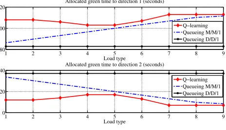
As illustrated in Fig. 3, the results show the allocated green time to each direction for each scenario. In D/D/1 queueing model, the optimal split from (9) is unaffected by the service rate. Therefore, the optimal split from the D/D/1 depends on the proportion of vehicle arrival rates only.

1 2 3 4 5 6 7 8 9

80 100 120

Allocated green time to direction 1 (seconds)

Load type

Q−learning Queueing M/M/1 Queueing D/D/1

1 2 3 4 5 6 7 8 9

0 20 40

Allocated green time to direction 2 (seconds)

Load type

[image:4.612.317.549.496.630.2]

Figure 3. Allocated green time to each direction

(5)

1 2 3 4 5 6 7 8 9 0

20 40 60 80 100

Effect of loading on the network throughput

Load type

Network throughput (percentage)

[image:5.612.309.550.72.202.2]

Figure 4. Network throughput comparison among Q-learning, Queueing M/M/1 and Queueing D/D/1

1 2 3 4 5 6 7 8 9

0 100 200

Link delay in direction 1 (seconds) Q−learning

Queueing M/M/1 Queueing D/D/1

1 2 3 4 5 6 7 8 9

0 1000 2000

Link delay in direction 2 (seconds) Q−learning

1 2 3 4 5 6 7 8 9

0 1000 2000

Average link delay from 2 directions (seconds)

Load type Q−learning

[image:5.612.61.303.72.204.2]

Figure 5. Link delay obtained from AIMSUN

significantly improved up to 3.2-14.8% from the D/D/1. Note that in the undersaturated conditions, the network throughput by both the M/M/1 and the D/D/1 also outperform the proposed CTM-based Q-learning algorithm. Fig. 5 explains why Q-learning performs well and badly in different traffic conditions. The link delay is generally known as the dif-ference between the time spent to travel along a particular road and the free flow travel time along the road. Fig. 5 illustrates the individual link delay for each direction and

1 2 3 4 5 6 7 8 9

0 50

Mean queue length in direction 1 (vehicles) Q−learning

1 2 3 4 5 6 7 8 9

0 100 200

Mean queue length in direction 2 (vehicles) Q−learning

1 2 3 4 5 6 7 8 9

0 100 200

Mean queue length from 2 directions (vehicles)

Load type Q−learning

[image:5.612.62.297.241.374.2]

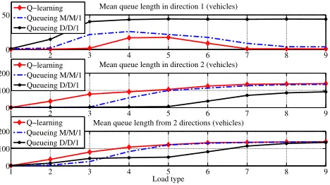
Figure 6. Mean queue length obtained from AIMSUN

1 2 3 4 5 6 7 8 9 0

50 100 150 200 250 300

Effect of loading on the average vehicle delay per completed trip

Load type

Average vehicle delay per completed trip

Figure 7. Average vehicle delay per completed trip comparison among Q-learning, Queueing M/M/1 and Queueing D/D/1

the average link delay from two directions. In each cycle time, the Q-learning has been allocated the green time more often to the direction that has higher vehicle arrival rates. However, in both queueing models, the allocated green time in each direction is directly proportional to the incoming trafﬁc demand of its direction. Therefore, by using Q-learning in the undersaturated conditions, the obtained optimal split leads the system to the wasted green scenario. However, the link delay of Q-learning performs well in the jamming conditions because the Q-learning can reduce the link delay from the higher vehicle arrival rates that dominate the overall link delay of the systems. As illustrated in Fig 6, the results for the mean queue length can be used explained with the same discussions as the link delay.

These three approaches share the common goal of min-imising the total network delay. Generally, the total network delay has been calculated from the difference of the time spent to complete a network trip and the free ﬂow travel time along the network path. For each vehicle, the average vehicle delay per completed tripAD can be calculated by

AD=

∀p(ALDp×CP Tp)

p CP Tp

, (17)

where ALDp is the average link delay in direction p and

CP Tp is the number of completed trips in direction p. In Fig 7, for the jamming condition, the reduction of the average vehicle delay per completed trip can be greatly reduced by up to 7.0-63.4% from the M/M/1 and can be signiﬁcantly reduced up to 18.9-80.7% from the D/D/1.

VI. CONCLUSION AND FUTURE RESEARCH DIRECTIONS

[image:5.612.62.296.536.667.2]

(6)

condition in comparison with the respective M/M/1 and D/D/1 approaches. Moreover, the average vehicle delay per completed trip can also reduce by up to 7.0-63.4% and by up to 18.9-80.7% in comparison with the respective M/M/1 and D/D/1 approaches.

In this paper, the basic assumptions are based on the M/M/1 model which is rather restricted, thus we are currently investigating other distributions. Furthermore, we are also investigating the scenario when the actual state (i.e. the number of vehicles) is concealed from the agent. In such case, the agent does not have a complete knowledge of the state of the system and must select a traffic signal under such a circumstance. In addition, the existing works related to Q-learning have not considered the scalability issues due to the limitation in terms state space explosion. However, we attempt to alleviate the explosion by employing state space quantisation and control traffic signal in such network scenarios. Methods to find the best possible traffic signal for the road traffic problems in a jamming condition become crucial. Therefore, the extension of the CTM-based Q-learning algorithm and its ability to deal with the jamming conditions will be reported in the forthcoming paper.

ACKNOWLEDGMENT

The authors would like to thank for support received from the Honours Program Scholarship from Electrical Engineer-ing Department of Chulalongkorn University and Thailand Graduate Institute of Science and Technology (TGIST), as-sociated with National Science and Technology Development Agency (NSTDA).

REFERENCES

[1] Xiao-Hua Yu and Allen R. Stubberud. Markovian decision control for trafﬁc signal systems.Proceedings of the 36th IEEE Conference on Decision and Control., 1997.

[2] G. F. Newell. The rolling horizon scheme of trafﬁc signal control.Transportation Research Part A: Policy and Practice., 32(1):39–44, 1998.

[3] P. B. Mirchandani and Z. Ning. Queuing models for analysis of trafﬁc adaptive signal control.IEEE Transactions on Intelligent Transportation Systems., 8(1):50–59, 2007.

[4] R. Wunderlich, C. Lui, I. Elhanany, and T. Urbanik. A novel signal-scheduling algorithm with quality-of-sevice provisioning for an isolated intersection. IEEE Transactions on Intelligent Transportation Systems., 9(3):536–547, 2008.

[5] Richard S. Sutton and Andrew G. Barto. Reinforcement Learn-ing: An Introduction. The MIT Press, 1998.

[6] B. Abdulhai and L. Kattan. Reinforcement learning: Introduc-tion to theory and potential for transport applicaIntroduc-tions.Canadian Journal of Civil Engineering., 30(6):981–991, 2003.

[7] C. Jacob and B. Abdulhai. Integrated traﬁc corridor control using machine learning. IEEE International Conference on Systems, Man and Cybernatics., 2005.

[8] S. Ritcher. Trafﬁc light scheduling using policy-gradient rein-forcement learning.The International Conference on Automated Planning and Scheduling., ICAPS, 2007.

[9] M. A. Wiering, J. Vreeken, J. Veenen, and A. Koopman. Simulation and optimization of trafﬁc in a city.IEEE Intelligent Vehicles Symposium., 2004.

[10] Y. Li, R. Wu, and W. Li. The coordination between trafﬁc signal control agents based on q-learning The 5th World Congress on Intelligent Control and Automation., 2004

[11] S. Lu, X. Liu, and S. Dai. Incremental multistep q-learning for adaptive trafﬁc signal control based on delay minimization strategy. Proceedings of the World Congress on Intelligent Control and Automation., WCICA, 2008.

[12] W. Kaige, Q. Shiru, and Z. Yumei. A stochastic adaptive control model for isolated intersections. IEEE International Conference on Robotics and Biomatics., 2008.

[13] Y.S. Hong, J.S. Kim, J.K. Son, and C.K. Park. Estimation of optimal green time simulation using fuzzy neural network. IEEE International Fuzzy Systems Conference Proceedings., 1999.

[14] M. C. Choy, D. Srinivasan, and R. L. Cheu. Cooperative, hybrid agent architecture for real-time trafﬁc signal control. IEEE Transactions on Systems, Man, and Cybernetics Part A:Systems and Humans., 33(5):597–607, 2003.

[15] A. Sadek and N. Basha. Self-learning intelligent agents for dy-namic trafﬁc routing on transportation networks. International Conference on Complex Systems., 2006.

[16] C.H. Shin and K.Choi Saturation ﬂow rate estimation under rainy weather conditions for on-line trafﬁc control purpose. ASCE Journal of Civil Engineering., 2(3):211-222, 2008.

[17] L. Klienrock. Queuing Systems Volume 1: Theory, 1975.

[18] C. F. Daganzo. The cell transmission model part II: Net-work trafﬁc.Transportation Research Part B: Methodological., 29b(2):79–93, 1995.