Multivariate Logistic Mixtures
Xiao Liu
TUMSchoolofEducation,andCentreforInternationalStudentAssessment,Arcisstrasse21,80333Munich,Germany
Copyright c2015 by authors, all rights reserved. Authors agree that this article remains permanently open access under the terms of the Creative Commons Attribution License 4.0 International License
Abstract
Logistic mixtures, unlike normal mixtures, have not been studied for their topography. In this paper we discuss analogs of some of the multivariate normal mixture results for the multivariate logistic distribution. We focus on graphical techniques that are based on displaying the elevation of the density on the ridgeline. These techniques are quite elementary, and carry full information about the location and relative heights of the modes and saddle points. Moreover, we turn to a technique that names II-Plot which denotes that the first differentiation of the second component density ratios the difference between the first differentiations of the second component density and the first component density.Keywords
Logistic Mixture, Multivariate Mode, Ridgeline, Pi-Plot1
Introduction
There is the work by Ray and Lindsay ([6]) on the key features of multivariate normal mixtures, including the deter-mination of the number of modes and general modality theorems. For the logistic distribution, on the other hand, such information seems to be lacking. The logistic distribution plays an important role in psychometrics for instance, for modeling item response functions (see [7]).
In this paper, we propose analogs of the multivariate normal mixture results for the multivariate logistic distribution (see [4]). The literature on determination of the number of modes in logistic mixture models has focused primarily on univariate mixtures. In fact, there is a simple description of modality when one is mixing two univariate components. Unlike the mixture of multivariate normal distributions (see [6]), for the logistic case it seems infeasible to express the ridgeline function explicitly. However, applying the implicit function theorem, we can prove that a unique explicit formula is possible locally. Moreover, we focus on displaying the elevation of the logistic mixture density on the ridgeline and address a technique called theΠ-plot, both of which carry important information about modality properties of the mixture.
We conclude with remarks about the similarities and differences between the multivariate normal and logistic distributions in regards to their mixture properties and conclusions thereof.
2
The Ridgeline Manifold
2.1
The
(
K
−
1)
-dimensional ridgeline manifold
AK-component mixture ofD-dimensional logistic distributions can be represented by the probability density function
g(x) =
K X i=1
πiφ(x;µi,si), x∈RD (2.1)
whereπiis the mixing proportion of componenti,πi∈[0,1], PK
i=1πi= 1, andφ(x;µ,s)is the density of a multivariate lo-gistic distribution with meanµand standard deviations. We will sometimes useφi(x)as shorthand notation forφ(x;µi,si), and callφitheith component density, where (following [4])
φi(x) =QDD!
j=1sij exp
−
D X j=1
(xj−µij)/sij
1 +
D X j=1
exp
−(xj−µij)/sij
−(D+1)
Definition 1. The(K−1)-dimensional set of points
sK=
(
α∈RK:αi∈[0,1], K X i=1
αi= 1 )
(2.3)
will be called the unit simplex. The functionx∗(α)fromsKintoRDwill be called the ridgeline function, which satisfies the
following condition
K X i=1
αi D X k=1
s−ik1
1−D+ 1
Eik
= 0 (2.4)
whereEik= 1 + e xk−µik
sik + exk
−µik
sik PD j6=ke
−xjsij−µij
.
The image of this map will be denoted byMand called the ridgeline surface or manifold. According to Lemma2(see AppendixA), we can get that Definition1is well-defined.
Theorem 1. Letg(x)be the density of aK-component multivariate logistic density as given by formula(2.1). Then all of
g(x)’s critical values, i.e. the values ofxsuch that∇g(x) = 0, are points inM.
Proof. Suppose that∇g(x∗) = 0, sox∗is a critical point. Then we have
K X i=1
πiφi(x∗)∇φi(x
∗)
φi(x∗)
= 0. (2.5)
If we let
αi=
πiφi(x∗)
PK
i=1πiφi(x∗)
, (2.6)
then obviously,0≤αi ≤1andPKi=1αi= 1. Further, note that
∇φi(x∗;µ,s)
φi(x∗;µ,s)
=−
D X k=1
s−ik1
1−D+ 1
Eik
. (2.7)
Thus from equation (2.4), we have that for every critical valuex∗there exists anαsuch that K
X i=1
αi D X k=1
s−ik1
1−D+ 1
Eik
= 0.
The above formula gives the theorem.
Remark 1. Due to the Taylor expansion(see AppendixB)until first order ata=−1from the right side of formula(2.2),
omitting the remainder, we can get that
φi(y) =QDD!
j=1sij
·
QD
j=1 −eyj
1−PDj=1eyjD+1. (2.8)
whereyj= (xj−µij)/sij.
Following formulae(2.5)and(2.6), we can get
K X i=1
αi∇φi(x
∗)
φi(x∗)
= 0. (2.9)
WhenD= 2, according to
∇φ(y)
φ(y) =
y1+y2+ 6e1−e(y1+y2) 2
1−e(y1+y2)y1y2
,
we obtain
K X i=1
αiny1+y2+ 6e
1−e(y1+y2)
2o
Corollary 1. Ifsik=si·, letDi=
QK j=1Ej
Ei , and
Fi=
D X k0=1
Fik0 = D X k0=1
QD k=1Eik
Eik0 ,
then the convex hull of(D + 1)DiFi contains the value of QK
i=1Ei at all critical points of the density g, whereEi = QD
k=1Eik.
Proof. Following formula (2.4), we can get K
X i=1
αis−i·1=
K X i=1
αis−i·1 D X k=1
D+ 1
Eik = K X i=1
αis−i·1(D+ 1)Fi
Ei =
(D+ 1)PKi=1αis−i·1DiFi QK
i=1Ei
.
Then
K Y i=1
Ei=
(D+ 1)PKi=1αis−i·1DiFi PK
i=1αis−i·1
. (2.11)
Thus the above formula gives the corollary.
2.2
The ridgeline elevation plot
The next step in our analysis is to consider the diagnostic properties of the elevation plot, which is a plot of the ridgeline elevation f unctiondefined by
h(α) =g(x∗(α)).
Remark 2. The positive and bounded density functionφi(x)characterized by the parameters(µi,si)in its second-order
Tay-lor expansion depends onx∈RDas a decreasing function of the Mahalanobis distance(x−µi)Tdiag(s2
i1, . . . , s2iD)−1(x− µi). This ties in with Remark 4 of Ray and Lindsay (2005), where these authors generalize the theorem to other families of multivariate distributions.
Due to second-order Taylor series approximation (see AppendixB),lφi, ofφiabouta=−1, omitting the remainder,
lφi(y) =
D!
QD j=1sij
·
e 2
DQD j=1 y
2
j + 1
1 +2ePDj=1 y2
j + 1 D+1
≤ QDD!
j=1sij
·
e 2
D
(maxj yj2+ 1
)D
e 2
D
(maxj yj2+ 1
)D ·
1
1 + e2PDj=1(y2
j + 1)
= QD D!
j=1sij
1 +e2D+2ePDj=1y2
j ,
whereyj = (xj−µij)/sij.
Remark 3. The density function oftdistribution withνdegrees of freedom
f(x;µ,Σ, ν) = Γ(
ν+D
2 )|Σ|
−1/2 (πν)D2Γ(ν
2) [1 + (x−µ)0Σ−1(x−µ)/ν]
1 2(ν+D)
(2.12)
where
Γν 2
:=
Z ∞
0
xν2−1e−xdx,
which follows [5], characterized by parameters(µ,Σ)depends onx ∈ RD as a decreasing function of the Mahalanobis
Example 1. Consider the logistic mixture withD= 2andK= 2, and with the parameters
µ1=
0 0
, s1=
1 0.5
,
µ2=
1 1
, s2=
1 0.5
, π1=π2=
1 2.
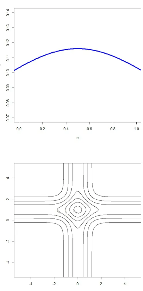
The corresponding ridgeline elevation functionh(α)is shown in Figure1. Following formula (2.4), we know
Gα(x1, x2) :=
α1
h
1− 3
E11
+ 21− 3
E12 i
+α2
h
1− 3
E21
+ 21− 3
E22 i
= 0
where
E11= 1 + ex1+ ex1−2x2, E12= 1 + e2x2+ e2x2−x1;
E21= 1 + ex1−1+ ex1−2x2+1, E22= 1 + e2(x2−1)+ e2x2−x1−1.
Definition 2. Let
di=Sα−1(vi−vK),
where for fixedαdefined the matrixSα=Pαis−i·1and vectorsvi=s−i·1
P k
1−D+1
Eik
. We can define a linear subspace of vectors that are orthogonal to the surface’s direction vectorsdiin an appropriate sense,
W={w:w0Sαdi= 0∀i= 1, ..., K−1}. (2.13)
Theorem 2. Ifw∈W, then along the path{x(α) +δw:δ∈R}the functiong(x)takes its maximum valuea atδ= 0.
Proof.
We know that the pointx(α)lies in one of the elliptical contours of the densityφi. According to formula (2.7), at this point the gradient inxof the densityφi(x)is proportional tovi, and soviis orthogonal to the contour. Thus, if we were to start atx(α)and travel in any directionworthogonal tovi, our path is in the support hyperplane to the elliptically shaped upper set{x:φi(x)≥φi(x∗(α))}. Using the fact that the ellipse ofφiis convex, our path lies outside the ellipse, and so in the set{x:φi(x)< φi(x(α))}, except for equality atx=x∗(α). This means, the point ofx∗(α)is a local maximum to φi(x)along any path orthogonal tovi.
Now, assume thatw∈W. It follows from the form ofdithat
w0(vi−vK) = 0. (2.14)
However, from the fomula (2.4), we havePαiv
i = 0, and soPαi(vi−vK) = −vK. Due to (2.13), we know that
w0vK = 0. Putting this together with (2.14) shows thatw0vi = 0fori = 1, ..., K.That is,w0 is orthogonal to everyvi, and hence, by the above paragraph, every component of the mixture densityg(x)is locally maximized along the given line
{x(α) +δw:δ∈R}atδ= 0, and thus, so isg(x).
Corollary 2. IfD≥K−1, then at a critical point ofh(α)whose second derivative matrix hasK−1negative eigenvalues
the functiong(x)will have a critical point whose second derivative matrix has an additionalD−K+ 1negative eigenvalues corresponding to the dimension of the orthogonal directionsw. Specially, forD > K−1, so that theh(α)plot is a true dimension reduction, theng(x)has no local minima, only saddlepoints and local maxima.
Proof.
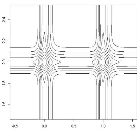
Figure 2.Ridgeline elevation for the bivariate logistic mixture of Example2along the ridgeline pathx∗(α), expressed as a function of parameterα. The
local maximum representing the mode of the density is visible nearα= 0.5.
3
Some Illustrative Examples
Example 2. The mixture logistic density withD= 3andK= 2, and the parameters
µ1=
0 0 0
, s1=
1 1 0.05
,
µ2=
1 1 1
, s2=
1 1 0.05
, π1=π2= 1 2.
Example 3. The mixture logistic density withD= 2andK= 3, and the parameters
µ1=
0 0
, s1=
1 0.05
,
µ2=
1 1
, s2=
0.05 1
,
µ3=
2 2
, s3=
1 0.05
, π1=π2=π3=
1 3.
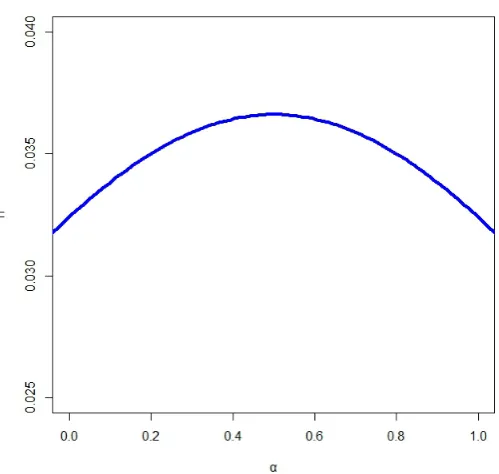
Figure3shows the contours of the density given in Example3.
Remark 4. More expressive detail for the two-dimensional plots of this section could have been obtained by displaying the
critical net of the density using, for example, the approximation techniques of Danovaro et al. [1]. This would show the maxima, saddlepoints and separatrices over the manifold region based on evaluating the elevation at a finite network of points.
Proof. First to prove that the logistic density is a Morse function. WhenD= 2, following formula (2.2),
φ= 2
s1s2 e−
x1−µ1 s1 −
x2−µ2 s2
1 + e−
x1−µ1 s1 + e−
x2−µ2 s2
[image:6.595.113.319.464.545.2]Figure 3.Density contour plot for the three component mixture density of Example3.
After calculation, we know that ∂2φ
∂x2 1
= 2
s3 1s2
e−x1
−µ1 s1 −
x2−µ2 s2
1 + e−x1
−µ1 s1 + e−
x2−µ2 s2
−3
− 18
s3 1s2
e−
x1−µ1 s1 −
x2−µ2 s2
1 + e−
x1−µ1 s1 + e−
x2−µ2 s2
−4
e−
x1−µ1 s1
+ 24
s3 1s2
e−
x1−µ1 s1 −
x2−µ2 s2
1 + e−
x1−µ1 s1 + e−
x2−µ2 s2
−5
e−2
x1−µ1
s1 , (3.1)
∂2φ
∂x1∂x2
= 2
s2 1s22
e−
x1−µ1 s1 −
x2−µ2 s2
1 + e−
x1−µ1 s1 + e−
x2−µ2 s2
−3
− 6
s2 1s22
e−
x1−µ1 s1 −
x2−µ2 s2
1 + e−
x1−µ1 s1 + e−
x2−µ2 s2
−4
e−
x1−µ1 s1
− 6
s2 1s22
e−
x1−µ1 s1 −
x2−µ2 s2
1 + e−
x1−µ1 s1 + e−
x2−µ2 s2
−4
e−
x2−µ2
s2 (3.2)
+ 24
s2 1s22
e−
x1−µ1 s1 −
x2−µ2 s2
1 + e−
x1−µ1 s1 + e−
x2−µ2 s2
−5
e−
x1−µ1 s1 −
x2−µ2 s2 ,
∂2φ ∂x2 2
= 2
s1s32 e−
x1−µ1 s1 −
x2−µ2 s2
1 + e−
x1−µ1 s1 + e−
x2−µ2 s2
−3
− 18
s1s32 e−
x1−µ1 s1 −
x2−µ2 s2
1 + e−
x1−µ1 s1 + e−
x2−µ2 s2
−4
e−
x2−µ2 s2
+ 24
s1s32 e−x1
−µ1 s1 −
x2−µ2 s2
1 + e−x1
−µ1 s1 + e−
x2−µ2 s2
−5
e−2x2
−µ2
s2 . (3.3)
Then the Hessian matrix is non-degenerate (invertible) at critical points. Thus, following [1], we get that this remark is given.
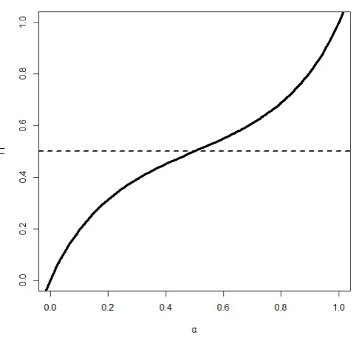
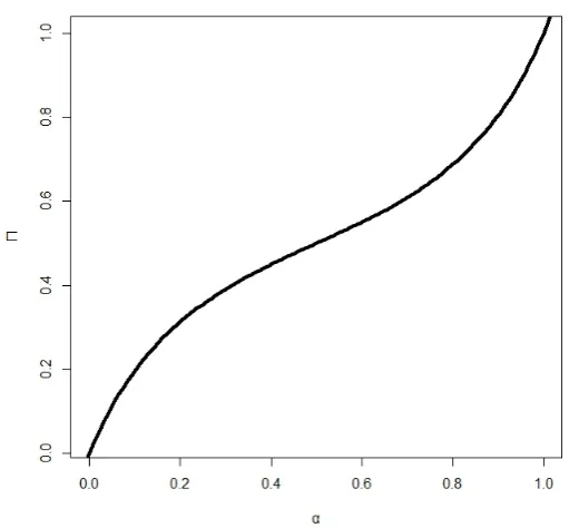
Figure 4.Π-plot of Example1.
4
The
Π
-PLOT
ForK = 2, considering the ridgeline curvex∗(α)defined in condition (2.4). Whenx∗(α)is a critical value ofh(α), it satisfies
h0(α) =πφ1(x∗(α))0+ (1−π)φ2(x∗(α))0 = 0, where ”0” denotes differentiation with respect toα.
Solving the above displayed equation forπ, and turning it into a function ofα, we get
Π(α) = φ
0
2(α)
φ02(α)−φ01(α). (4.1)
We can also derive the following simple calculation formula forΠ(α):
1 Π(α) =
φ02(α)−φ01(α)
φ02(α) = 1 + 1−α
α
φ1(α)
φ2(α), (4.2)
which can be verified by formulae (2.5) and (2.6).
As an example, let us examine the Π-plot (graph ofΠ(α)) of the two-component bivariate logistic mixture with two modes given in Example1. As the mixing proportion in Example1isπ= 0.5, we would draw a horizontal line across the
(α,Π(α))plot (Figure4) at heightπ= 0.5. This line crosses the curve once. Among these, nearα= 0.5correspond to the one mode, as was verified by the ridgeline elevation plot (see Figure1).
For Example2, similar with Example1we can find (see Figure5), at heightπ= 0.5, nearα= 0.5corresponds to one mode, as was verified by the ridgeline elevation plot (see Figure2).
5
Analytic tools for detecting modality
5.1
The curvature function
In this section, we look more deeply into the properties of theΠfunction.
Considering back to the above section, the first differentiation ofΠfunction with respect toαis
Π0(α) =−φ
00
2(α)φ01(α)−φ001(α)φ02(α)
(φ02(α)−φ01(α))2 . (5.1)
Figure 5.Π-plot of Example2.
As following we will use the curvature functionκ(α)defined by
κ(α) =φ
00
2(α)φ01(α)−φ001(α)φ02(α)
φ2(α)φ1(α) . (5.2)
5.2
Properties of the curvature function
κ
(
α
)
Now we turn to give two properties ofκ(α).
Lemma 1. (Two components, two dimensions, equal variance). In the equal variance case(s1=s2),κ(α)reduces to the
following expression
q(x) =φ002(x)φ01(x)−φ001(x)φ02(x). (5.3)
The logistic mixturegwill be bimodal if and only ifπ∈(π1, π2), where
1
πi = 1 +
1−αi αi
φ1(αi)
φ2(αi) (5.4)
and theαiare the solutions in[0,1]ofq(x) = 0.
Proof. According to that the case is in two dimensions,
Π0(α) = 0
⇒φ002(α)φ01(α)−φ001(α)φ02(α) = 0 (5.5) where
φ0(α) =
∂φ ∂x1
+ ∂φ
∂x2
˙
x(α);
and
φ00(α) =
∂2φ
∂x2 1
+ 2 ∂ 2φ
∂x1∂x2 +∂
2φ
∂x2 2
˙
x(α) +
∂φ ∂x1
+ ∂φ
∂x2
¨
Then
φ002(α)φ01(α)−φ001(α)φ02(α) =
∂φ
1
∂x1 +∂φ1
∂x2
˙
x(α)
∂2φ 2
∂x21 + 2 ∂2φ
2
∂x1∂x2 +∂
2φ 2
∂x22
˙
x(α) +
∂φ
2
∂x1 +∂φ2
∂x2
¨
x(α)
−
∂φ2
∂x1 +∂φ2
∂x2
˙
x(α)
∂2φ1
∂x2 1
+ 2 ∂ 2φ
1
∂x1∂x2 +∂ 2φ 1 ∂x2 2 ˙
x(α) +
∂φ1
∂x1 +∂φ1
∂x2
¨
x(α)
= φ002(x)φ10(x) ˙x2(α)−φ001(x)φ20(x) ˙x2(α)
(5.6) Thus
φ002(x)φ01(x)−φ001(x)φ02(x) = 0. (5.7)
Corollary 3. Letgbe the mixture of two logistic densities with meansµ1andµ2and standard deviations1ands2=σs1.
gis bimodal if and only ifπ∈(π1, π2), where
1
πi = 1 +
1−αi αi
φ1(αi) φ2(αi)
and correspondingly theαiare the solutions in[0,1]of
φ002(x)φ01(x)−φ001(x)φ02(x) = 0. (5.8) Specially, the one dimensional case of logistic mixture is in the preprint paper ”A Note On The Convex Combination Of Two 1-, 2-, 3-, and 4-Parameter Logistic Item Response Functions”, which is according to [8].
6
Conclusion
In this paper, we have proposed a technique for the topography of multivariate logistic mixtures. This is performed by the ridgeline functionx∗(α)and theΠ-Plot. Unlike with the case of multivariate normal mixtures, it is difficult to express the ridgeline functionx∗(α)explicitly. However we can prove that we can get a unique explicit formula ofx∗(α)through the implicit function theorem. Thus we can obtain theΠ-Plot even if we can not get the ridgeline contour plot whenK≥3.
Future developments of the work described here consists of improving over the technique for displaying the contour plot whenK = 3following the Taylor expansion to take into account of the solution of ridgeline equation. The mathematical expression of the constructive implicit function theorem in logistic case is also very interesting. Otherwise, an application of this work can be used in PISA (Programme for International Student Assessment) analysis.
A
Definition 1 is well-defined
Lemma 2. The left side of formula(2.4)is satisfied implicit function theorem.
Proof. Let
ψ(x) :=
K X i=1 αi D X k=1
s−ik1
1−D+ 1
Eik
for any fixedk, we can get ∂ψ ∂xk = K X i=1 αi
s−ik1D+ 1 E2
ik
· dEik
dxk + D X k06=k
s−ik10 D+ 1
E2
ik0
·dEik0
dxk = K X i=1 αi
s−ik2eyk D+ 1
1 + eyk+ eykPD j6=ke−yj
2
1 +
D X j6=k
e−yj
−
D X k06=k
s−ik10s−ik1
D+ 1
1 + eyk0+ eyk0PD j6=k0e−yj
2e yk0e−yk
= K X i=1
αi(D+ 1)s−ik1
s−ik1eyk
1 + eyk+ eykPD j6=ke−yj
2
1 +
D X j6=k
e−yj
−
D X k06=k
s−ik10eyk0
1 + eyk0+ eyk0PD j6=k0e−yj
2e
−yk
According to the arbitrariness ofµikandµik0, we know that for∀xkandxk0, we can getyk =yk0. So formula (A.1) are not permanently equal to0, fork= 1,· · · , D.
Following implicit function theorem (see page 89 of [3]), formula (2.4) can overlap locally with the graph ofx=x∗(α), wherex∗(α)is an explicit function.
B
Taylor Expansion
The Taylor expansion of a real-valued functionf(x)that is infinitely differentiable at a real numberais the power series f(a) +f
0(a)
1! (x−a) +
f00(a) 2! (x−a)
2+f(3)(a) 3! (x−a)
3+· · ·.
which can be written in the more compact sigma notation as N
X n=0
f(n)(a)
n! (x−a)
n+o (x−a)N
wheren!denotes the factorial ofn,o (x−a)N
denotes that the remainder is higher order infinitesimal of(x−a)N and f(n)(a)denotes thenth derivative offevaluated at the pointa.
C
Implicit function theorem
Let f : Rn+m → Rm be a continuously differentiable function, and letRn+mhave coordinates (x,y). Fix a point
(a,b) = (a1, ..., an, b1, ..., bm)withf(a,b) =c, wherec∈Rm. If the matrix
Y=
∂f1
∂y1(a,b) · · · ∂f1 ∂ym(a,b) ..
. . .. ...
∂fm
∂y1(a,b) · · · ∂fm ∂ym(a,b)
is invertible, then there exists an open setUcontaininga, an open setV containingb, and a unique continuously differentiable functiong:U →V such that
{(x, g(x))|x∈U}={(x,y)∈U×V|f(x,y) =c}.
REFERENCES
[1] E. Danovaro, L. De Floriani, P. Magillo, M. M. Mesmoudi and B. Abraham. Morphology-driven simplification and multiresolution modeling of terrains. In Proc. Eleventh ACM International Symposium on Advances in Geographic Information Systems, 63–70, ACM Press, New York, 2003.
[2] L. De Floriani and P. Magillo. Multiresolution mesh representation: Models and data structures.Tutorials on Multireso-lution in Geometric Modelling, 363–418, Springer-Verlag, 2002.
[3] O. Forster. Analysis 2.Vieweg Tuebner, 8th. Version, 2008.
[4] H. J. Malik and B. Abraham. Multivariate logistic distributions. The Annals of Statistics, 1(3):588–590, 1973.
[5] D. Peel and G. J. McLachlan. Robust mixture modelling using thetDistribution.Statistics and Computing, 10:339–348, 2000.
[6] S. Ray and B. G. Lindsay. The topography of multivariate normal mixtures. The Annals of Statistics, 33(5):2042–2065, 2005.
[7] M. D. Reckase. Multidimensional Item Response Theory.Springer, New York, 2009.