Munich Personal RePEc Archive
Modeling Overstock
Fernandes, Rui and Gouveia, Borges and Pinho, Carlos
Universidade de Aveiro
8 June 2010
Modeling Overstock
Rui Miguel Costa Fernandes ([email protected]) University of Aveiro
Joaquim José Borges Gouveia GOVCOPP / University of Aveiro
Joaquim Carlos da Costa Pinho GOVCOPP / University of Aveiro
Abstract
Two main problems have been emerging in supply chain management: the increasing pressure to reduce working capital and the growing variety of products. Most of the popular indicators have been developed based on a controlled environment. A new indicator is now proposed, based on the uncertainty of the demand, the flexibility of the supply chains, the evolution of the products lifecycle and the fulfillment of a required service level. The model to support the indicator will be developed within the real options approach.
Keywords: overstock, stock management, real options
Literature review
Most of the studies done pointed the sourcing flexibility as a way to deal with the uncertainty from the demand side. For Antanies (2002), the performance of the working capital must be solved considering the impact of uncertainty of demand in the level of inventory, using a vendor management inventory system combined with components of the products. For Jian et al. (2004) and Forslund et al. (2007), the way to deal with demand uncertainty is based on the definition of parameters of the safety stock. Hadley (2004), presented two perspectives in inventory management: the cycle inventory and the safety inventory. Tan (2008), considered that the safety stocks are kept to minimize the forecast mistakes. Borgonovo et al. (2007) pointed a sensitivity analysis to deal with uncertainty, also based on the input parameters of the traditional models. For Lapide et al. (2008), the way to deal with uncertainty is by increasing the number of buffers, using the variability buffering law (inventory, capacity, time).
Nevertheless the improvements done on traditional safety stock, the demand is assumed as being deterministic. However, some studies have pointed a stochastic approach, which of the most common are: the base stock model, stochastic multi-echelon systems and strategic safety stock. The main assumptions of these approaches are based on the fact that there are no fixed costs and on the decision between assuming holding inventory costs and stock-out costs.
prioritized base-stock policy can be used to control the production to meet exogenous Poisson demands. He used a matrix analytical method.
The multi-echelon systems are based on the definition of a stock level in each stage of a chain, using the net-lead-time. Pearson (2003) presented an equilibrium solution to the two-echelon problem. Bollapragada et al. (2004) introduced a new concept: the cost weighted stock levels.
The study of Graves et al. (2000), points the strategic safety stock as way to optimize the inventory levels, modeled as a spanning tree under uncertain demand. Schmit (2008) made a reference to over-stock inventory (cycle stock plus safety stock).Workman et al. (2009) has pointed three classifications for the safety stock: safety stock demand, supply and strategic.
To solve the problem of uncertainty, Tan et al. (2009) proposed, applying for Monte Carlo simulation, the use of a reserved stock to prospective future demand, based on customer preference classification.
Sodhi et al. (2009) proposed to extend the linear programming model of deterministic supply-chain planning, to take demand uncertainty and cash flows into account for the medium term.
Moole et al. (2004), stated that the way to deal with uncertainty is getting and working data (decision support system). Also Sheffi (2001) stated that the share of information along the chain can improve the reaction to demand uncertainty. Tan (2007) defended the forecasting methods advance demand information. Based on the rolling horizon flexibility, Walsh et al. (2007) examined the way to minimize the impact of uncertainty of the demand, in a discrete event simulation model, and Matuyama et al. (2009) defended the forecast systems improvements. Ryu et al. (2009) add the importance of sharing information between players.
Lusa et al. (2008) used a multistage stochastic optimization model in the study of the relation between the resources planning optimization and the demand uncertainty. For Mukhopadhyay et al. (2009), there are two ways to deal with the demand uncertainty: by flexibility in sourcing or adjusting the yield rate of the internal production resources.
For Marvel et al. (2007) and Bish at al. (2009), the manufacturer can avoid the impact of demand uncertainty by developing a better ordering prioritization system from the retailer. Graman et al. (2010) split demand into two parts: predicted demand and non predicted demand. The paper presented by Handfield et al. (2009) introduced the concept of penalty costs for orders not fulfilled. Song et al. (2010) presented the reorder point and order quantity, based on optimal policy parameters to deal with demand uncertainty but limited to one single item which, according to Hemmelmayr et al. (2010), does not consider the relevant product mix uncertainty.
Real options
The origin of the term “real option” go back to 1977 and was due to professor Stewart
capacity to estimate the future unit price as there is no forward price market) (Boyer et al, 2003).
Overstock as a real option
When a company faces a stochastic demand, in scale and mix, it is required an efficient resources management, also as the adaptation to restrictions in the capacity of the supply chain, according to the required volume and time. In this situation, the managers should choose options that are able to minimize the risk of inventory and the risk of not having the item available, in face of a demand manifestation.
The evolution done in the past, applying for shorter lead-times, shorter invested capital and shorter costs, changed the supply chain in order to become leaner. But, from Sept 11th 2001, a new feeling of uncertainty rose and are changing the form of managing the supply chain. The physical flow of materials depends on the availability of infrastructures (from the firm, the suppliers and the public global providers). Dual source strategies rise to minimize the risk associated with a disruption. Companies
complement the “just in time” concept with the “just in case” concept (Sheffi, 2001),
which means a revaluation of the need of safety stock, both on source and client delivery. The planning should change from a push centralized strategy to a pull market oriented strategy (Sengupta, 2004). This explains the need of changing the tools that support the stock management, from a historical data support to a forecast data based, within limitations of resources and minimizing the risk.
Most of the applications of the term overstock were related with excess of stock. In 2007, new approaches were done introducing the concept of obsolescence cost (Emsermann et al., 2007) and overstock risk (Jia-zhen et al., 2007). Recently, Ding et al. (2008) made an approach to overstock, considering it as an avoidable and shared loss between supply chain players.
Model assumptions
Considering an installed capacity and restrictions in the use of an outsource option, it’s
possible to use an overstock option. This means the use of an option to increase stock above a maximum position. This option should be based on the demand uncertainty, in quantity and mix, to allow risk minimization of a negative answer to a client request. Overstock option allows risk minimization of product stock-out, for which the company assumes a lead time, and it forces the minimization of the out-of-mix stock risk for excessive inventory. It was proved by Schmit (2008), that there is a relation between supply uncertainty and inventory level and for Stalk (2008), the inventory level must be linked with scale and product portfolio. The uncertainty affects the demand (as a stochastic process) but also the combination of items (as a logistic basic unit part) – this
is what we can call as “the mix effect”.
In the present model, overstock is defined as the excess of stock above maximum stock. This excess, allows the minimization of sales lost risk, due to restrictions in the available capacity of the supply chain or of the driver resources. To apply to this concept, an item classification is required, changing the traditional “ABC” perspective, to a more complex classification, regarding the actual context of uncertainty, like the mix variety and diversity, products lifecycle decrease and the consequent innovation process increase. Considering these arguments, products should not be treated in the same way.
“A’s” is the terminology for those items representing more than 80% of the gross sales value. These items can follow a make to stock procedure, depending on the existing push or pull strategy. They can be called as fast movers. “B’s” for items that fulfill the gross sales value gap between 80% and 95%. They can follow an assembly to order procedure, based on available components, in a stage where standardization is possible. They can be defined as movers. These items should be storable using sales forecast, with low risk. “C’s” is the name for the items with a low rotation. They are used to
promote sales of A’s or B’s items (mix attraction); that is why there should be small batch quantities in stock. They can be identified as slow movers. “Sp’s” for those items that are assigned to one client or market segment, nevertheless the use of a specific or shared distribution channel. The stock risk tends to infinitive. We can define them as specific products (niche oriented). “N’s” is the name for the new items. They are identified as new products or phase-in products. There’s a high risk exposure. “P’s” is the designation of the items that are in the maturity stage. In this stage, there should be a preparation of the tools to allow a minimum phasing-out cost. For these items, risk is a variable with high probability to occur. They are known as products with potential risk. O’s for the items in the “death” stage. For these items, the risk is a constant.
Overstock calculation
Overstock should be calculated by item group, using the previous classifications (A, B, C, S, N, P and O).
[image:5.595.110.489.486.611.2]Definition of variables: lead Time definition in weeks = Lt; Sales historical value for n weeks = Vn; Variance coefficient = α (depending on the item category); Number of weeks = n; Actual stock value = S; Actual book of orders value for n weeks = δn; Sales value forecast for n weeks = βn and Profit margin (sales unit price - stock unit cost) / sales unit price = θp.
Table 1 – Overstock expression
Item classification
Overstock expression
A and B
n n n i i i i i AB ti n i i B B A A i S p n n
L 1 ; 1... ; 1...
1 1
C and Sp
n n n i i i i i CSp ti n i i Sp Sp C C i S p n n
L 1 ; 1... ; 1...
1 1
N i n n
i i i i N ti n i i N N i S p n n
L 1 ; 1...
1 1
P and O 1 ; 1... ; 1... ; 0
1 1
n n ti
n i i i i i PO ti n i i L O O P P i S p n Vn
L
Modeling overstock as a real option
Main assumptions of the model: the items classification is an auxiliary process, the information of the output of this process depends only on the firm, the stocks refer only to manufactured items and the demand (quantity) is a stochastic variable (the firm does not have any influence on quantity and sales price – is a price taker).
Basic assumptions of the model: the products can be analyzed individually, according to a defined classification; any demand not fulfilled from stock is lost at moment t, the lead times are fixed and known and it is not consider the impact of lost market share in period t+1 due to a disruption in near time t.
Valuing the flexibility
The decision is about the level of overstock value (stock above the previous existing level). For the model is important a cost function and eventually the capacity constraints, as this is the limitation for future orders fulfillment. The model will not consider efficiency in the use of the available resources (this issue should be treated in the manufacturing flexibility). The capacity constrains will not be considered. We assume it is not relevant to the decision process. The overstock value should be calculated according to each product classification. The classification will be done considering the product lifecycle and will be treated as an independent auxiliary process.
Source of uncertainty
The source of uncertainty is the demand (quantity), that we are going to represent by
“D”. Company cannot influence the sales price with the level of overstock. The possibility of have available material to deliver will not change the sales price behavior. The evolution of the demand is the most important input for the option valuation. We assume that the demand of each product category is stochastic and follows a geometric Brownian motion (assumption done also by Pindyck (1988); Tannous (1996); Bengtsson (2001)). The demand process can be presented as:
dD = αDdt + σDdz (1)
Where dz =
t dt ; Є(t) ≈ N(0,1); α = instantaneous drift; σ = volatility; dz = increment of a winner process; where Є(t) is a serially uncorrelated and normally distributed random variable.From equation (1) we can state that the demand (D) is log-normally distributed with a variance that grows with the time horizon (also an assumption of the model presented by Bengtsson (2001)). The demand is modeled as a continuous process. We assume that all the production and stock policy is make-to-stock.
Decision rules and payoff
Variable meaning: h = stock aging factor; D = demand in quantity for the item category;
v
c = variable production cost of a single unit; pv= unit sales price; 1 – S = stock out rate
for item class; K = value calculated as a function of the stock out rate (normal distribution); S = required service level for item category: % of the quantity fulfilled on the required date; Lt = lead time definition; j = Weighted average cost of capital,
reported and adjusted to period t (simplification); = average stock unit cost; It1 = existing inventory level in the beginning of period n; n= period n (between t-1 and t); Mv = (pv - cv). D; n= period n (between t-1 and t); ks = cost of holding stocks for each
item for period
t1n t
.If we study one overstock option, which expires at time t, and gives us the option to adjust the stock level, if the benefits exceed the costs for changing the stock level, respecting the maximum allowed capital, the value of the option at time t (Ω(t)) can be written as:
1
1
1
t s Mv S It
k h j K L D
The value of the overstock option is the expected terminal value of the condition:
t max D Lt K 1 j h ks Mv 1 S It1,0
(3)
Where “DLtK” represents the stock allowed using the traditional approach;
“Mv
1S
” represents the loss margin related to sales not fulfilled on time and“
s
k h
j ” represents the opportunity cost of the invested capital, the risk of
obsolescence and the weight of the handling costs on the average stock unit cost. s.t.
t Ct
0 (4)
t
C = maximum invested capital value allowed in stocks for time t.
In this form, the overstock can be expressed as a European call option, where
j h k
M
S
K L
D s v
t
1 1
is the value of the underlying asset (A). The
actual stock level It1 can be treated as the exercise price (E). An overstock manufacturing order should take place if Ω(t) ≥ 0. The overstock option gives the right to increase stock level above the existing one, for each product category, and expires in time t.
Boundary conditions:
Absorbing barrier: 0; when
t 0 Expiration optimal condition:
,0
1 1
max D Lt K j h ks Mv S It 1
(5)
Value matching at *
t (optimal overstock level) :
1
1
1
t s Mv S It
k h j K L D (6)
Valuing the option
The value of an overstock option, for time t, must satisfy the following differential equation: 0 . 2 1 . . 2 2
2
r D d d dD d D (7)
Valuation model: numerical example
analyzes the performance of stocks management based on historical data. But, considering the volatility of the demand distribution, of more than 20%, the firm needs to anticipate the stocks level to avoid disruptions. The problem is how to anticipate within a certain required level of performance. The demand is considered a stochastic variable. Demand volatility assumption = 0,25.
Table 2: Parameters value for the numerical example
Factor Description Value Unit
D demand quantity 262.051 m2
It-1 stock value at the beginning of period 4.849.145 euros
h stock aging factor 0,002 coefficient
cv variable production cost of a single unit 5,000 €/sku
pv unit sales price 15,000 €/sku
S required service level 95,000 %
j Weighted average cost of capital 0,500 %/month
Lt Lead time definition 1,5 months
ks holding stock cost/unit for the period 0,263 €/sku
θ average stock unit cost 7,500 €/sku
Results of the model
Ωt = Overstock value (option value) = 323.714 euros.
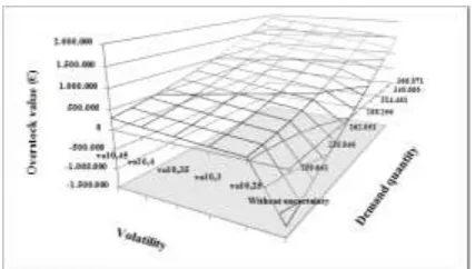
The impact on the stocks level due to the introduction of a stochastic variable will be analyzed. The first approach will be the analysis of the impact of the growth of the demand on the overstock value, for different volatility parameters.
Figure 1: Demand quantity variation, demand volatility and the overstock value
Figure 2: Lead time, demand volatility and the overstock value
When the lead time increases there is an additional need of time to answer for a request. This period of time, demands a high level of stock to buffer the gap between the output time of the physical flow and the orders date.
Figure 3: Obsolescence rate, demand volatility and the overstock value
The obsolescence rate states for the average stock that can go throw a phase out stage in a short period of time. There is a high risk perception. For this reason, the overstock allowed decreases as this rate increases. To avoid more risk, the firm must develop the activities to support the phase out process in a proper way.
Conclusions
The goal of this study was the determination of the overstock level allowed, in order to satisfy the service level requirements also as the adequacy of the invested capital on stocks. The common way to analyze stocks is based on historical data and treats all the items in the same way, not respecting the products lifecycle evolution.
The numerical models normally used, do not adapt to changes in the demand, because they tend to follow the past tendencies. In this way, overstock comes as an alternative tool for stocks management. The calculation of the adjusted overstock level can be supported on the real options approach, mainly based on two drivers: the demand - as an uncertainty variable input, and the overstock - as a flexible indicator within the supply chain. In the overstock decision process, there is a relation between the increase of the uncertainty and the need to increase the stocks’ value. The model also states that, in the absence of uncertainty, the stocks level can be calculated by the traditional formula, which means no overstock. If there is no flexibility in management, the stock value is influenced by a conditional parameter which can also have the same result as using the traditional approach.
When applying the real options approach (ROA) to the overstock calculation, we can
environments. The ROA is a way to support the decision process, in order to maximize the required value improvement.
The contribution of this work is the enlargement of the tools used for stocks management, respecting the actual need of future oriented based decisions, as a consequence of the increasing in the uncertainty of the markets, also as the need to account for the product lifecycle evolution. It was proved that the overstock level can be calculated and used, and there is an optimal value to be fulfilled. It was also proved the link between the demand quantity and volatility with the stock value, the lead-time and service level definitions and the product lifecycle impact, based on the use of the obsolescence factor.
The model was aimed to introduce the volatility of the demand on the stock value calculation. Nevertheless, there is also an important impact of the items classification, as it can gives a better view about the study of the best process to apply for the
demand’s behavior. A future application of the concept can count with an additional and more elaborated level of uncertainty, based on the products lifecycle evolution. The lifecycle evolution can influence directly the lead times and the service level definitions. There should also be considered the impact of the capacity constraints, along the chain, as an uncertainty source. The overstock value can also help managers in smoothing the resources used, allowing an increase in the relation between effectiveness and costs.
References
Antanies, J. (2002), “Recognizing the effects of uncertainty to achieved working capital efficiency”,Pulp & Paper. San Francisco, Vol. 76, Iss. 7, pp. 46, 4 pgs.
Bengtsson, J. (2001), “Manufacturing flexibility and real options”,Department of Production Economics, IMIE, Linköping Institute of Technology, S-581 83, Linköping, Sweden.
Bish, E.; Liu, J. and Suwandechochai, R.(2009), “Optimal Capacity, Product Substitution, Linear
Demand Models, and Uncertainty”, The Engineering Economist. Norcross: Apr-Jun, Vol. 54, Iss. 2, pp. 109.
Bollapragada, R.; Rao, U.S. and Zhang, J. (2004), “ Managing two-stage serial inventory systems under demand and supply uncertainty and customer service level requirements”, IIE Transactions, 36, pp.73–85.
Borgonovo, E. and Peccati, L. (2007), “Global sensitivity analysis in inventory management “, International Journal of Production Economics. Amsterdam, Jul, Vol. 108, Iss. ½, pp. 302. Boyer, M.; Christoffersen, P.; Lasserre, P. and Pavlov, A. (2003), “Value Creation, Risk Management,
and Real Options”,CIRANO, Université de Montréal, McGill University, UQÀM, Simon Fraser University.
Ding, D. and Chen, J. (2008), “Coordinating a three level supply chain with flexible return policies”, Omega, Oxford, Vol. 36, Iss. 5, Oct, pp. 865.
Emsermann, M. and Simon, B. (2007), “Optimal Control of an Inventory with Simultaneous Obsolescence”, Interfaces. Linthicum, Sep/Oct , Vol. 37, Iss. 5, p. 445 (12 pages).
Forslund, H. and Jonsson, P. (2007), “The impact of forecast information quality on supply chain
performance”,International Journal of Operations & Production Management, vol 27, n 1, pp. 90-107, 98-104.
Gertner, R.; Rosenfield, A. (1999), “How real options lead to better decisions; [Surveys edition]” Financial Times. London (UK): Oct 25, p. 06.
Graman,G. A. (2010), “A partial-postponement decision cost model”, European Journal of Operational Research, Amsterdam, Feb 16, Vol. 201, Iss. 1; pp. 34.
Graves, S. C.; Willems, S. P. (2000), “Optimizing strategic stock placement in supply chains”, Manufacturing & Service Operations Management, Informs, Vol 2, Nº 1, Winter, pp 68-83. Hadley, S. W. (2004), “A Modern View of Inventory”,Strategic Finance. Montvale, Vol. 86, Iss. 1,
p.30,6pgs.
Handfield, R.; Warsing, D. and Wu, X. (2009), “ (Q,r) Inventory policies in a fuzzy uncertain supply chain environment”, European Journal of Operational Research, Amsterdam, Sep 1, Vol. 197, Iss. 2, pp. 609.
Jian, L. and Ma, S. (2004), “Research on values of safety factor coordination under random supply”, International Journal of Services Technology and Management, Geneva, Vol. 5, Iss. 1; pp. 90. Jia-zhen, H.; Jian-jun, Z.; Jin, Z. (2007), “Influence of Overstock Risk on Buy Back Strategy in Supply
Chain”,Wireless Communications, Networking and Mobile Computing, WiCom. International Conference on, 21-25 Sept., pp 4657 – 4661.
Lapide, L. (2008), “How Buffers Can Mitigate Risk”, Supply Chain Management Review. New York, Apr, Vol. 12, Iss. 4, pp. 6, 1 pgs.
Lusa, A. ; Corominas, A. and Muñoz, N. (2008), “A multistage scenario optimisation procedure to plan annualised working hours under demand uncertainty”, International Journal of Production
Economics, Amsterdam, Jun, Vol. 113, Iss. 2, pp. 957.
Marvel, H. P. and Wang, H. (2007), “A generic approach to measuring the machine flexibility of manufacturing systems Inventories, Manufacturer Returns Policies, and Equilibrium Price Dispersion under Demand Uncertainty”, Journal of Economics & Management Strategy, Cambridge, Winter, Vol. 16, Iss. 4, pp. 1031.
Matuyama, K.; Sumita, T. and Wakayama, D. (2009), “Periodic forecast and feedback to maintain target inventory level”, International Journal of Production Economics, Amsterdam, Mar, Vol. 118, Iss. 1, pp. 298.
Moole, B. R. and Korrapati, R. B. K. (2004), “A Decision Support System Model for Forecasting in Inventory Management using Probabilistic Multidimensional Data Model (PMDDM)”, Allied Academies International Conference. Academy of Information and Management Sciences. Proceedings. Cullowhee, Vol. 8, Iss. 2, pp. 35, 6 pgs.
Mukhopadhyay, S. K. and Ma, H. (2009), “Joint procurement and production decisions in remanufacturing under quality and demand uncertainty”,International Journal of Production Economics, Amsterdam, Jul, Vol. 120, Iss. 1; pp. 5.
Pearson, M. (2003), “An equilibrium solution to supply chain synchronization”, Centre for Mathematics and Statistics, Management School, Napier University, Edinburgh, EH11 4BN, UK IMA Journal of Management Mathematics, 14(3), pp.165-185.
Pindyck, R. S. (1988), “Irreversible Investment, Capacity Choice, and the Value of the Firm”,The American Economic Review, Vol. 78, No. 5, pp. 969-985.
Ryu, Seung-Jin; Tsukishima, T.; Onari, H. (2009), “A study on evaluation of demand information-sharing methods in supply chain”, International Journal of Production Economics, Amsterdam, Jul, Vol. 120, Iss. 1, pp. 162.
Sengupta, S. (2004), “The top 10 supply chain mistakes”, Supply Chain Management Review, New York, Vol. 8, Iss. 5, Jul/Aug, pp. 42.
Sheffi, Y. (2001), “Supply Chain Management Under The Threat of International Terrorism”,The International Journal of Logistics Management, 12, 2, pp. 1-11.
Sodhi, ManMohan S. and Tang, C. S. (2009), “Modeling supply-chain planning under demand uncertainty using stochastic programming: A survey motivated by asset-liability management”, International Journal of Production Economics, Amsterdam, Oct, Vol. 121, Iss. 2, pp. 728.
Song, Dong-Ping (2008), “Stability and optimization of a production inventory system under prioritized base-stock control”, International Shipping & Logistics Group, The Business School, University of Plymouth, UK.
Song, Jing-Sheng; Zhang, H.; Hou, Y. and Wang, M. (2010), “The Effect of Lead Time and Demand Uncertainties in (r, q) Inventory Systems”, Operations Research. Linthicum, Jan/Feb, Vol. 58, Iss. 1, pp. 68, 16 pgs.
Stalk, G. (2008), “Confronting the Growing Supply Chain Crisis”, Business Finance, Loveland, Vol. 14, Iss. 6, Jun, pp. 28-29.
Tan, T. (2008), “Using Imperfect Advance Demand Information inForecasting”, Department of Technology Management, Eindhoven University of Technology, IMA Journal of Management Mathematics Advance, February 16.
Tannous, G.F. (1996), “Capital Budgeting for Volume Flexible Equipment”, Decision Sciences, 27, No. 2. pp. 157-184.