http://dx.doi.org/10.4236/jmp.2013.412205
The Large Numbers in a Quantized Universe
Yan Ryazantsev*
52, 43 Dimitrova Street, Zagoryansky, Shchelkovo District, Moscow, Russia Email: [email protected]
Received October 3, 2013; revised November 5, 2013; accepted November 29, 2013
Copyright © 2013 Yan Ryazantsev. This is an open access article distributed under the Creative Commons Attribution License, which permits unrestricted use, distribution, and reproduction in any medium, provided the original work is properly cited.
ABSTRACT
The article relates to a decades-old problem of the mysterious coincidence between various large numbers of the mag-nitude ranging from 1040 to 10120 which sometimes appears in cosmology and quantum physics. Using well known
clas-sical relations as well as the ideal Schwarzschild solution the exact relations of various large numbers, the fine structure constant and π were found. The new largest number law is claimed. The hypothetical approximations of the Hubble parameter—68.7457(82) km/s/Mpc, Hubble radius—14.2330(17) Gly, and some others were proposed. The exact formulae supporting P. Dirac’s large number hypothesis and H. Weyl’s proposition were found. It is shown that all major physical constants with the length dimension (from the Compton wave length of universe through the Planck and atomic scale up to the Hubble sphere radius) could be derived from each other, and the table of the specific conver-sion rules has been developed. The model shows that the Eddington-Weinberg relation can be transformed to precise identity. It is shown that both Bekenstein universal entropy bound and Bekenstein-Hawking Black Hole entropy bound are proportional to the largest number doubled.
Keywords: Large Numbers Hypothesis; Hubble Sphere; Eddington Number; Cosmological Constant
1. Introduction
The problem of Large Numbers dates back decades. The first problem statement and attempts at resolving it can be found in the studies by H. Weyl [1-3] and Sir A. Eddington [4,5], who drew attention to the incredibly large numbers of the dimensionless physical constants found in the cosmology, electrodynamics and quantum mechanics. The magnitude of these constants is so big
10 , 10 , 10 , 1020 40 80 120
as compared with the con-ventional mathematical constants, like π3.14 and Euler’s constant e 2.71 , that boggles imagination as P. Davies [6] noted.
The first of the two most popular dimensionless large numbers is the classical ratio between the gravitational force and the electromagnetic force in any given distance, called by H. Weyl [2] “even more mysterious than the fine structure constant ”:
42 4.16 10
e e
DF
g g
f r
N
f r
(1)
were:
2 2 0
1 4π
e
q f
r
(2)
2
2 e g
m
f G
r
(3)
The second is the ratio of the universe radius to the classical electron radius:
40
4.63 10
DR
e e
R c
N
r Hr
(4)
where H is Hubble’s constant, re—classical electron
radius, R—Hubble sphere radius or radius of event
horizon, rg—gravitational electron radius, fe—electros-
tatic force between two electrons at a distance r, 0—
permittivity of vacuum, q —electron charge, fg —
gravitational force between two electrons at a distance r, G—Newton gravitational constant, me—electron mass.
The proximity of magnitude of re
R and
g e
r
r values
led H. Weyl to the idea that the incredible weakness of gravitational interaction may be due to the ratio of the electron and the universe radiuses or to the total quantity of particles in the universe—the Eddington number [5].
We refer everybody interested in the history of stu- dying the problem of large numbers to the reviews by S. Ray, U. Mukhopadhyay, P. P. Ghosh [7] and K. A. Tomilin [8].
The hypothesis by P.A.M. Dirac is one of the best known hypotheses put forward to explain the problem of large numbers [9-11]. He supposed that the reason for appearance of great magnitudes of dimensionless values is their reliance on the equally large value, so-called “cosmological time”. This led P. Dirac to the hypothesis of dependence of the gravitational constant and the universe mass on time:
1
G T
(5)
2
M T (6)
where M is the mass of universe, T is cosmological
time.
The idea of time-varying constants was developed, in particular, by E. A. Milne [12]. To establish the ratios and laws between modern values of the fundamental constants, we suggest studying values of large numbers at the current point of time, without taking into account their time derivative. P. Dirac’s assumption that New- ton’s gravitational constant and the mass of universe are not true constants but change over time gave rise to an array of scientific discussions, experimental and theore- tical studies devoted to verification of the fundamental constants in subsequent decades. No reliable proofs of variability of the physical constants were found yet.
In this article, we will use the Hubble time, the parameter inverse to the Hubble constant, as approxi- mation of the cosmological time:
1
T H
(7)
We referred to the simplest mathematics in narrating the article; however, the results we obtained provide quite good approximation to the most precise and generally accepted values of physical parameters, such as
e
m and re, taking into account their uncertainties. In
particular, CODATA 2010 [13] as well as the measure- ments of Mission Planck 2013 [14] were used.
2. Revealing the Large Numbers Ratios
To discover the correlation between large numbers in our epoch, let’s begin with the well known vacuum solution to the Einstein’s equations for spherically symmetric and static universe. According to Schwarzschild’s solution, the universe’s radius R that coincides with the Black
Hole radius with the mass of M is determined by a
well-known formula (Schwarzschild radius):
2
2GM R
c
(8)
On the other hand, we know the formula for the electron gravitational radius that includes more or less precisely measured physical values:
2 e g
Gm r
c
(9)
Therefore, the formula for the classical electron radius that uses G can be easily obtained from (8) and (9):
2
DF e
e
N Gm
r c
(10)
We will not discuss now if the value of the classical electron radius has any real physical significance. It is enough that it is one of the energy status representations of an electron, a particle with the minimum self-energy among all charged particles.
For transition to energy values, we will use a large mass number introduced by H.Weyl:
e U
M
e U e
E M
N
m E
(11)
where 2
U
E Mc —the universe self-energy, Eem ce 2
—the electron self-energy, U h
Mc
—Compton wave
length of the universe, e
h mc
—Compton wave length
of the electron.
By dividing (8) by (10), one can get the following ratio:
2
e DF e
R M
r N m (12)
Thus, we obtain the precise correlation among the three large numbers out of (4), (11) and (12):
2NM NDFNDR (13)
Besides the above large numbers, we will use a large energy number NW representing the ratio of the
universe’s self-energy EU and “the minimum vacuum
energy” EW as proposed by J. Casado [15]:
U W
W
E N
E
(14)
where
2
W
hc
E H
R
—quantum of energy with wave
length 2πR, h—Planck’s constant;
We will also need another large number equal to the cube of NDR value:
3 3 3
U DR
e
R
N N
r
(15)
Introduction of a new designation for a large number
U
number has a particular and substantial value. One of the simplest classical interpretations of this number: “the large number NU represents the total number of, say,
‘elementary clusters’ in the universe—the ratio between volume VU of ball-like universe and the region Ve
folded by sphere of radius re”. Taking into account that
this number has the greatest magnitude as compared with other large numbers
10122
, we suggest calling it “theLargest number”.
3. The Largest Number Law and Revealing
of Dirac’s Proportionalities
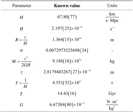
[image:3.595.309.538.100.198.2]Now let us use well known physical parameters with their uncertainties (see Table 1). The parameters listed in
Table 1 enable us to calculate large numbers values (see
Table 2). To obtain NDF, we use (10):
2
1 e DF
e
r c N
G m
(16)
We should pay an attention to the very close values of
U
N and NW of the magnitude 121
10
. The ratio between this two large numbers is
3.185(36)
U x
W
N n
N
(17)
This is quite remarkable, taking into account the extremely large magnitudes of the numbers involved. Therefore, we can assume that this ratio is not just a coincidence but some specific physical law. In order to reveal the meaning of the ratio (17) one can rewrite it as follows:
2
3 3 2
3 3 2 2
2π 1 2π
W e e e
x
U
e e e
E m c r m
R R R
n
E M
r r Mc R r
(18)
[image:3.595.57.286.543.736.2]By simply grouping the cosmological parameters in
Table 1. Known physical parameters.
Parameter Known value Units H 67.80 77 s Mpckm H 2.197 25 10 18 s1
c R
H
1.364 15 10 26 m
0.0072973525698 24 -
3
2
c M
GH
9.188 10 10 52 kg
e
r 2.8179403267 27 10 15 m 1
T H
4.551 52 10 17 s
T 14.43 16 Gyr G 6.67384 80 10 11
2 2
N m kg
Table 2. Calculated Large numbers values.
Parameter Value
DF
N 4.16589 50 10 42
DR
N 4.842 55 10 40
U
N 1.135 39 10 122
M
N 1.009 11 10 81
W
N 3.564 81 10 121
the left-hand side, and the quantum ones in the right- hand one the ratio (17) can be transformed into the following relation:
2 2
universe electron
1 e x
e
m M n
R r
(19)
The question is—what kind of a phisical law the last equation represents?
In order to find out the answer we would like to propose quite a simple classical model. We can apply the classical approach because we are dealing with constant macroscopic physical parameters and those ratios. Let us consider a really large number of non-interacting quanta. All quanta are moving in all directions with a speed of light, i.e. there are photons. Obviously, the set must be
confined inside the Black Hole with a radius R If the
total energy of the whole quanta set is equal to EU. We
have to conclude that absolutely every photon must be reflected by the sphere’s bound in certain time. In other words the inner side of the Hubble sphere plays a role of an ideal diffusely reflecting surface. In a period of time
T R c we will see that ultimately all quanta had
experienced a reflection from the bound. It means that the inner side of the Hubble sphere looks like a Lam- bertian light emitter for an internal observer. Thus the constant radiant emittance from the inner side of our Black Hole can be expressed by the formula:
3 2
1 4π
4π
U U
E
W MH
R T
(20)
Now let us consider the observer-a spherical body in a vacuum with radius r0R placed at the center of the
Hubble sphere. The observer will find out a constant isotropic quanta flow that is falling to an every surface area S from a spatial hemisphere above the area.
According to the Lambert’s cosine law a radiant energy flux in through the area S (i.e. irradiance) will
be:
π
2π
2
0 0 cos sin in
U W
S
(21)where is the angle between the beam and a line normal to the surface area S.
of our spherical observer:
in in
S
S S
(22)
2 0 sin
S r
(23)
where and are spherical coordinates of the area
S
on observer’s surface. Thus:
π
2π π 2π 2
2
0 0 0 0 0 cos sin sin
in WU r
(24) The last integral (24) can be simplified as follows:
2
2 2 0
0 2
4π π U
in U
E r r W
T R
(25)
The total amount of energy Etot entered inward (or
reflected by) the observer during the period of time T
is:
2 tot in tot
E T m c (26)
where mtot is a total mass which our observer should
have at present time if he absorbs (or reflects) the incoming energy flux in completely. Thus we can
write down the following equation:
2 2
2 2
0
πMc m ctot
R r (27)
Now, making a comparison of the Equations (27) and (19) one would ultimately conclude that if the coefficient
x
n in the (19) equals exactly to π then mtot r02 must
be equal to 2 e e
m r . Thus:
2 2
universe electron
1
π e e
m M
R r
(28)
Using (4), (11) and (28), we immediately obtain a noteworthy ratio between Weyl-Eddington-Dirac large numbers :
2 π
DR M
N N (29)
Hence, we can obtain the formula for the universe mass via the Hubble time:
2 2
2
2 2
π π
e e
e e
m R m c
M T
r r
(30)
The last one represents the proportional relation between M and T2 which was hypothesized by P.
Dirac almost 80 years ago.
As we see from (29), both fundamental constants and π are deeply involved in large number relations and thus we can assume that it is an evidence that cosmological and quantum parameters of our model of the universe are closely connected through geometry.
The above Equations (13) and (29) readily yield the correlation of the best known large Weyl-Eddington-Di- rac numbers, which include both the geometrical cons- tant π and the fine structure constant :
πNDF 2NDR
(31) This correlation is very notable. It enables one to calculate the approximations for Hubble sphere radius and the Hubble parameter via the correlation of gra- vitational and electrostatic forces:
1 π
2 DF e
R N r (32)
2
π
DF e
c H
N r
(33)
Now let us introduce the “big” angular momentum of the Hubble sphere measured along any given direction
:
MRc
(34)
Thus, multiplying both sides of the Equation (28) by
U
cN , we would propose the exact Largest number law in the following form:
π U
N (35)
The total sum of NU fundamental quanta of the
angular momentum in universe equals exactly to the angular momentum of the Hubble sphere multiplied by
π. This is a direct consequence of geometrical Lambert’s cosine law and rotational symmetry of space (conser- vation of angular momentum).
The following expression, as well as expressions (29) and (35), represent just another form of this law:
π
U M DR
N N N (36)
With the help of large numbers ratios and Largest number law, one can get various representations of the Newton constant of gravitation G using initial expres-
sion:
2 2 0
1 1
2 4π
e DR
M e
q N
G
N m
(37)
The most elegant cases, in our opinion, are:
2 2
0
8
e
DR e
q G
N m
(38)
and:
2 2 2 3 2
3
π π
2 8π 2
e e
e e e
r c h r c
G
m R m R m T
(39)
The last one represents the reverse proportional re- lation between G and R, which was hypothesized by
H.Weyl and between G and T which was hypo-
By means of (39), one can get representation of the cosmological constant :
4 2 3 2 2 2
8π 6 6 π 3
2
U M
DR
G GM N
c c R N R R
(40)
where U U
U
E
V
—energy density of the universe.
The last one represents the de Sitter space—a va- cuum solution of Einstein’s equation with cosmological constant-for the 4-dimensional case. Hence, we can ob- tain the formula for the cosmological constant via the fine structure constant , Weyl-Eddington-Dirac large number NDF, classical radius of electron re and
π:
212
π
DF e
N r
(41)
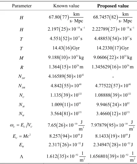
4. Calculations
The ratios between large numbers as described in Sec- tions 2 to 3 enable us to calculate many cosmological parameters in the proposed model. The calculations has been carried out (by using the constants , ,r m c Ge e, , ,π)
as follows: h N, DF,Ee, then NDR, then
, , , ,
U M
N N R H T , then M N, W,EW and then EU.
[image:5.595.59.285.467.738.2]The results of calculations of the constants based on referential data and information from the most recent measurements are shown in Table 3.
Table 3. Proposed values based on the the Largest number law.
Parameter Known value Proposed value H 67.80 77 s Mpckm 68.7457 82 s Mpckm H 2.197 25 10 s 18 1 2.22789 27 10 s 18 1 T 4.551 52 10 s 17 4.48853 54 10 s 17 T 14.43 16 Gyr 14.2330 17 Gyr M 9.188 10 10 kg 52 9.0606 22 10 kg 52
R 1.364 15 10 m 26 1.345629 16 10 m 26
DF
N 4.16589 50 10 42 -
DR
N 4.842 55 10 40 4.77522 57 10 40
U
N 1.135 39 10 122 1.08888 39 10 122
M
N 1.009 11 10 83 9.9465 24 10 82
W
N 3.564 81 10 121 3.4660 12 10 121
U E VU U
10
3
J 7.65 26 10
m
10
3
J 7.97879 95 10
m
2
U
E Mc 8.257 94 10 J 69 8.1433 19 10 J 69
W
E 2.317 26 10 J 52 2.34947 28 10 J 52
52
2
1 1.612 35 10
m
52
2
1 1.656801 39 10
m
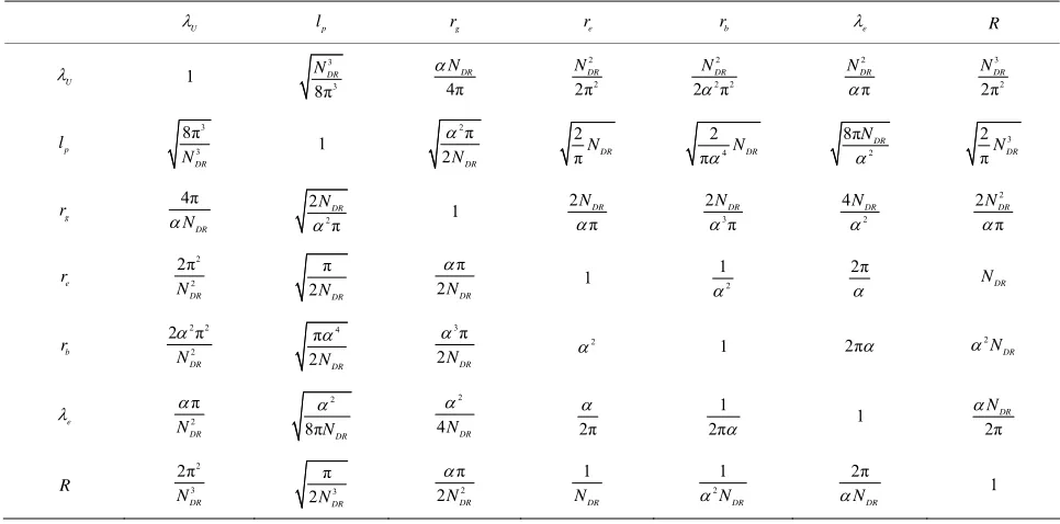
The ratios of large numbers described in the previous sections enable to link the Hubble volume radius and other constants with the length dimensions, including such parameters as the electron gravitational radius and the Planck’s length. All such constants can be calculated one from the other, via the fine structure constant , Weyl-Eddington-Dirac large numbers NDF or NDR
and π. The Tables 4 and 5 show the mutual conversion
ratios of the constants—from the Compton wave length of the universe to the Hubble sphere radius. To obtain the value of the top line parameter, one should multiply the initial parameter in the respective column by the formula in the cell at their crossing.
In Table 5, one can find one more elegant expre-
ssion-the ratio between largest and smallest distances in universe-radius of the Hubble sphere and the Compton wave length of the entire universe. It is proportional to the Largest number:
2
1
2π U
U
R
N
(42)
5. Examples of Applying the Large Number
Ratios
The previous sections contain a rather simple derivation of the inter-dependence of all main large numbers. The Largest number law that links the Weyl-Eddington-Dirac numbers enable validation of whether the known hypo- thetic equations and inequations conform to the large numbers combination we proposed or not. Below are several examples.
Example 1. J. Teller proposed [16] an interesting ratio
between Planck’s values, the fine structure constant and Hubble’s cosmological parameter:
1 8π exp
p p
p
H
m Hc t H
l
(43)
where 8π4G
c
—Einstein constant, m l tp, ,p p—Planck
units.
Having very large magnitude 1060, the left and
right parts of the formula give us values which differ from each other by only 1.5%. It is really remarkable but it is about 70 times more uncertain than other values calculated by us earlier:
1 32 π3 1
8πp e e 0.98588 12
U
t H
N
(44)
Table 4. Calculating parameters with a length dimension via NDF.
U
lp rg re rb e R
U
1 3 3
64 DF N 2 8 DF
N 2 2
8 DF N 2 8 DF
N 2 π
4
DF
N 3π 3
16
DF
N
p
l 3643
DF
N
1 NDF
DF
N
NDF3
2
4πNDF
3 3
π
2 NDF
g r 2 8 DF N DF N
1 NDF 2
DF
N
2πNDF
2 π 2 DF N e
r 2 2
8 DF N 1 DF N 1 DF
N 1 2
1 2π π 2 DF N b r 2 8 DF N 3 DF N 2 DF N 2
1 2π π 3
2
DF
N
e
24
π
DF
N 4π2
DF N
2πNDF
2π
1
2π 1
2
4
DF N
R 3 3
16
πNDF
3 2 3
4
πNDF
2
2
πNDF
2
πNDF
3
2
πNDF
2
4
DF
N
1
where lp—Planck length, rb—Bohr radius.
Table 5. Calculating parameters with a length dimension via NDR.
U
lp rg re rb e R
U
1 3
3 8π DR N 4π DR N 2 2 2π DR N 2 2 2 2 π DR N 2 π DR N 3 2 2π DR N p l 3 3 8π DR N 1 2π
2NDR
2
πNDR 4
2
π NDR 2
8πNDR
3
2
πNDR
g
r 4π
DR N 2 2 π DR N 1 2 π DR N 3 2 π DR N 2
4NDR
2 2 π DR N e r 2 2 2π DR N π
2NDR
π
2NDR
1 12
2π
NDR
b r 2 2 2 2 π DR N
π 4
2NDR
3π
2NDR
2 1 2π 2
DR N e 2 π DR N 2
8πNDR
2
4NDR
2π
1
2π 1 2π
DR N R 2 3 2π DR N 3 π
2NDR
2
π
2NDR
1 DR N 2 1 DR N 2π DR N 1
are even further from the reality.
Example 2. There is known Eddington-Weinberg
approximate relation [17]:
2 3
p
HGcm
(45) where 1.672621777 17 10
27kgp
m —proton mass
(CODATA 2010).
Using the approximation of H calculated above
(Table 3) one can get the ratio, which is quite far from
expected 1.0:
2
3 0.000264629 45 1
p H
Gcm
(46)
[image:6.595.55.538.384.623.2]the large number ratios to this hypothetical formula:
2
3 3
2
π
e
H Gcm
(47)
Example 3.
J. Bekenstein proposed [18] universal entropy bound for a complete physical system whose total mass-energy (in our case) is EU, and which fits inside a sphere of
radius R. Applying the large numbers ratios, we can get
the universal entropy bound value:
2π
2π 2π 2
U U
B W U
W
kE R E
S k kN kN
c E
(48)
Where k is Boltzmann constant.
On the other hand, the Bekenstein-Hawking entropy bound for the Black Hole with radius R is:
3 2 π
BH
kc R S
G
(49)
By dividing (48) by (49) and using (8) one can get:
4 2
2 U 2 1
B BH
E G
S MG
S c R c R (50)
The last one says that both Bekenstein universal entropy bound and Bekenstein-Hawking Black Hole entropy bound have the same value in our model and equal exactly to 2kNU:
122
99 J2.17776 78 10 3.0067 11 10
K
B
S k (51)
Using the large number ratios it is also easy to express the Hawking radiation EH of our Black Hole with
energy EU via Largest number NU or Hubble
parameter:
3
8π 4 4π 4π
U W
H H
U
E E
c H
E T k
GM N
(52)
where TH is Hawking radiation temperature.
6. Discussion and Conclusions
The two currently prevailing physical theories, i.e. quan-
tum mechanics and the general relativity, describe the reality very precisely, each in its range of energy and spatial scale. It is presumed that sometimes in the future, the value of NDF will be obtained in theory directly as
a direct result of consolidation of gravitation with other known interactions, strong and electroweak.
The fruitless attempts at explaining the proximity of
DF
N and NDR resulted in a broad application of the
term of “coincidence” that somehow highlights the randomness of the event. As shown in previous sections
it is not random.
As we see, the large number ratios proposed in the
article provide the powerful means for finding relations among various information and physical parameters of our model universe. However, it does not help answer the main question: where do these enormous numbers come from in physics? Hopefully, the law and hypotheses proposed in this article will let find the correct answer in the foreseeable future.
The ratios we suggested impose rather many stringent limitations on the way physical constants may change over time. We must note that the sharply tuned combi- nation of large numbers, including the mentioned appro- ximations for Hubble time T, mass of the universe M
and Hubble limit R correspond to the values of the
very precisely measured physical constants of quantum scale. Looking at (39) and (40), it is obvious that the gravity is closely connected with the Hubble radius, Hubble time and the properties of electron. However, there are rather reliable measurements that establish a very low limit for the Newton constant change rate in the long-term
< 1%
. Thus, if Hubble parameters ,T Rvaries with time then the corresponding variation of or/and electron energy 2
e
m c should preserve the cons-
tancy of G.
If the entire universe energy EU comprises (or once
comprised) quantums of the minimum energy EW, we
should make the conclusion that number (14) is a natural number. The same is true about (15). Hence, we can establish the hypothesis that all large numbers in the real
(not infinite) universe should be naturals or rationals.
However, the denominator and the numerator in these fractional numbers are so great that one can confidently presume the real large numbers approximate some per- fect limit of fundamental importance infinitely closely. Taking into account the transcendentalism of (29), (31) and (35), we dare to express one more hypothesis: all Large numbers are infinitely approaching their limits and these very limits are transcendent mathematical constants.
The Schwarzschild solution is one of the well known models of our universe, representing a Black Hole. Avoiding creation of new essences, we just consider the interaction between internal radiation and a small sphe- rical observer. It appears that such a simple model re- veals a lot of interesting identities and conservation laws. For example, the value of 2
0 tot
m r should be conserved
for a sphere with a radius r0. Furthermore we found that
identity mtot me is valid for a sphere with classical
electron radius re.
The last derivation allowed us to propose a list of exact ratios between well known Eddington-Weyl-Dirac large numbers which are listed in Table 2. The ratios (30)
form.
Using these large numbers ratios we have claimed the new Largest number law (35) which is based on Lam- bert’s cosine law and the rotational symmetry of space. It is quite important that this law precisely unites the major cosmological and quantum parameters of our universe. It could be interpreted as follows: our universe comprises of the mathematically determined number of elementary spatial clusters which can be matched up to energy quan- ta and angular momentum quanta. We should note that basic parameters of our model universe have been ob- tained form the properties of electron, speed of light and fine structure constant.
If Equations (13), (28) and (31) are valid inside the Hubble sphere, which is very probable, we should make a conclusion that all cosmological parameters are fully and unambiguously determined by quantum and mathe- matical constants. Simply put, all of us are very likely to live in an extremely precisely self-tuned quantized uni- verse.
REFERENCES
[1] H. Weyl, Annalen der Physik, Vol. 359, 1917, pp. 117-
145.
[2] H. Weyl, “The Open World Yale,” Oxbow Press, Oxford, 1989.
[3] H. Weyl, “Space Time Matter,” Methuen, Dover, 1952. [4] A. S. Eddington, “The Math. Theory of Relativity,” Cam-
bridge University Press, Cambridge, 1924.
[5] A. S. Eddington, “Fundamental Theory,” Cambridge Uni-
versity Press, Cambridge, 1946.
[6] P. C. W. Davies, “The Accidential Universe,” Cambridge University Press, Cambridge, 1982.
[7] S. Ray, U. Mukhopadhyay and P. P. Ghosh, Large Num- ber Hypothesis: A Review, 2007.
[8] K. A. Tomilin, Issledovaniya po Istorii Fiziki i Mekhaniki,
Vol. 141, 1999.
[9] P. A. M. Dirac, Nature, Vol. 139, 1937, p. 323.
[10] P. A. M. Dirac, Proceedings of the Royal Society A, Vol.
165, 1938, p. 199.
[11] P. A. M. Dirac, Nature, Vol. 1001, 1937.
[12] E. A. Milne, Proceedings of the Royal Society A, Vol. 158,
1937, p. 324.
[13] P. J. Mohr, B. N. Taylor and D. B. Newell, The 2010 CODATA Recommended Values of the Fundamental Phy- sical Constants, National Institute of Standards and Tech- nology, Gaithersburg, 2011.
http://physics.nist.gov/constants
[14] C. Planck, P. A. R. Ade, N. Aghanim, C. Armitage-Ca- plan, M. Arnaud, et al., Planck 2013 Results, Cosmologi- cal parameters, 2013.
[15] J. Casado, Connecting Quantum and Cosmic Scales by a Decreasing-Light-Speed Model, 2004.
[16] E. Teller, Physical Review, Vol. 73, 1948, pp. 801-802.
[17] S. Weinberg, “Gravitation and Cosmology,” Wiley, New York, 1972.
[18] J. D. Bekenstein, Physical Review D, Vol. 23, 1981, pp.