Munich Personal RePEc Archive
Maximum Likelihood Estimation of the
Multivariate Normal Mixture Model
Boldea, Otilia and Magnus, Jan R.
University of Tilburg
2009
Online at
https://mpra.ub.uni-muenchen.de/23149/
Maximum likelihood estimation of the
multivariate normal mixture model
∗
Otilia Boldea
Jan R. Magnus
May 2008. Revision accepted May 15, 2009
Forthcoming in:
Journal of the American Statistical Association, Theory and Methods Section
Proposed running head:
ML Estimation of the Multivariate Normal Mixture Model
Abstract: The Hessian of the multivariate normal mixture model is de-rived, and estimators of the information matrix are obtained, thus enabling consistent estimation of all parameters and their precisions. The usefulness of the new theory is illustrated with two examples and some simulation experi-ments. The newly proposed estimators appear to be superior to the existing ones.
Key words: Mixture model; Maximum likelihood; Information matrix
1
Introduction
In finite mixture models it is assumed that data are obtained from a finite collection of populations and that the data within each population follow a standard distribution, typically normal, Poisson, or binomial. Such models are particularly useful when the data come from multiple sources, and they find application in such varied fields as criminology, engineering, demography, economics, psychology, marketing, sociology, plant pathology, and epidemi-ology.
The normal (Gaussian) model has received most attention. Here we con-sider an m-dimensional random vector x whose distribution is a mixture (weighted average) of g normal densities, so that
f(x) = g X
i=1
πifi(x), (1)
where
fi(x) = (2π)−m/2
|Vi|
−1/2
exp{−1
2(x−µi)
′ V−1
i (x−µi)} (2) and the πi are weights satisfying πi > 0 and Piπi = 1. This is the so-called ‘multivariate normal mixture model’. The parameters of the model are (πi,µi,Vi) fori= 1, . . . , gsubject to two constraints, namely that theπi sum to one and that the Vi are symmetric (in fact, positive definite).
The origin of mixture models is usually attributed to Newcomb (1886) and Pearson (1894), although some fifty years earlier Poisson already used mixtures to analyze conviction rates; see Stigler (1986). But it was only after the introduction of the EM algorithm by Dempster et al. (1977) that mixture models have gained wide popularity in applied statistics. Since then an extensive literature has developed. Important reviews are given in Tit-terington et al. (1985), McLachlan and Basford (1988), and McLachlan and Peel (2000).
There are two theoretical problems with mixtures. First, as noted by Day (1969) and Hathaway (1985), the likelihood may be unbounded in which case the maximum likelihood (ML) estimator does not exist. However, we can still determine a sequence of roots of the likelihood equation that is consistent and asymptotically efficient; see McLachlan and Basford (1988, Sec. 1.8). Hence, this is not necessarily a problem in practice. Second, the parameters are not identified unless we impose an additional restriction, such as
see Titterington et al. (1985, Sec. 3.1). This is not a problem in practice either, and we follow Aitken and Rubin (1985) by imposing the restriction but carrying out the ML estimation without it.
The task of estimating the parameters and their precisions, and formu-lating confidence intervals and test statistics, is difficult and tedious. This is simply because in standard situations with independent and identically distributed observations, the likelihood contains products and therefore the loglikelihood contains sums. But here the likelihood itself is a sum, and therefore the derivatives of the loglikelihood will contain ratios. Taking ex-pectations is therefore typically not feasible. Even the task of obtaining the derivatives of the loglikelihood (score and Hessian matrix) is not trivial.
Currently there are several methods to estimate the variance matrix of the ML estimator in (multivariate) mixture models in terms of the inverse of the observed information matrix, and they differ by the way this inverse is approximated. One method involves using the ‘complete-data’ loglikeli-hood, that is, the loglikelihood of an augmented data problem, where the assignment of each observation to a mixture component is an unobserved variable coming from a prespecified multinomial distribution. The advan-tage of using the complete-data loglikelihood instead of the incomplete-data (the original data) loglikelihood lies in its form as a sum of logarithms rather than a logarithm of a sum. The information matrix for the incomplete data can be shown to depend only on the conditional moments of the gradient and curvature of the complete-data loglikelihood function and so can be readily computed; see Louis (1982). Another method, in the context of the original loglikelihood, was proposed by Dietz and B¨ohning (1996), exploiting the fact that in large samples from regular models, twice the change in loglikelihood on omitting that variable is equal to the square of the t-statistic of that variable; see McLachlan and Peel (2000, p. 68). This method was extended by Liu (1998) to multivariate models. There is also a conditional bootstrap approach described in McLachlan and Peel (2000, p. 67).
In this paper we explicitly derive the score and Hessian matrix for the multivariate normal mixture model, and use the results to estimate the infor-mation matrix. This provides a twofold extension of Behboodian (1972) and Ali and Nadarajah (2007), who study the information matrix for the case of a mixture of two (rather theng) univariate (rather than multivariate) normal distributions. Since we work with the original (‘incomplete’) loglikelihood, we compare our information-based standard errors to the bootstrap-based standard errors which are the natural small-sample counterpart.
We find that in correctly specified models the method based on the ob-served Hessian-based information matrix is the best in terms of root mean squared error. In misspecified models the method based on the observed ‘sandwich’ matrix is the best.
This paper is organized as follows. In Section 2 we discuss how to take account of the two constraints: symmetry of the variance matrices and the fact that the weights sum to one. Our general result (Theorem 1) is formu-lated in Section 3, where we also discuss the estimation of the variance of the ML estimator and introduce the misspecification-robust ‘sandwich’ ma-trix. These results allow us to formally test for misspecification using the Information Matrix test (Theorem 2), discussed in Section 4. In Section 5 we present the important special case (Theorem 3) where all variance matri-ces are equal. In Section 6 we study two well-known examples based on the hemophilia data set and the Iris data set. These examples demonstrate that our formulae can be implemented without any problems and that the results are credible. But these examples do not yet prove that the information-based estimates of the standard errors are more accurate than the ones currently in use. Therefore we provide Monte Carlo evidence in Section 7. Section 8 concludes. An Appendix contains proofs of the three theorems.
2
Symmetry and weight constraints
Before we derive the score vector and the Hessian matrix, we need to discuss two constraints that play a role in mixture models: symmetry of the variance matrices and the fact that the weights sum to one. To deal with the symmetry constraint we introduce the half-vec operator vech(·) and the duplication matrixD; see Magnus and Neudecker (1988) and Magnus (1988). LetV be a symmetricm×mmatrix, and let vechV denote the 12m(m+1)×1 vector that is obtained from vecV by eliminating all supradiagonal elements ofV. Then the elements of vecV are those of vechV with some repetitions. Hence, there exists a uniquem2×1
2m(m+1) matrixD, such thatDvechV = vecV. Since
The weights πi must all be positive and they must sum to one. We maximize with respect to π = (π1, π2, . . . , πg−1)
′
and set πg = 1−π1− · · · −
πg−1. We have
dlogπi =a
′
idπ, d2logπi =−(dπ)
′ aia′
i(dπ), (3) where
ai = (1/πi)ei (i= 1, . . . , p−1), ag =−(1/πg)ı, (4)
ei denotes the i-th column of the identity matrix Ig−1, and ı is the (g−
1)-dimensional vector of ones. The model parameters are then π and, for i= 1, . . . , g,µi and vechVi. Writing
θi =
µi vechVi
,
the complete parameter vector can be expressed as θ= (π′ ,θ′
1, . . . ,θ
′
g)
′
.
3
Score vector, Hessian and variance matrix
Given a samplex1, . . . ,xnof independent and identically distributed random variables from the distribution (1), we write the loglikelihood as
L(θ) = n X
t=1
logf(xt).
The score vector is defined by q(θ) =Ptqt(θ), where
qt(θ) = ∂logf(xt)
∂θ = vec(q
π
t,q1t, . . . ,q g t),
and the Hessian matrix by Q(θ) = PtQt(θ), where
Qt(θ) = ∂
2logf(xt)
∂θ∂θ′ =
Qππt Qπt1 . . . Qπgt Q1tπ Q11t . . . Q1tg
..
. ... ...
Qgπt Qgt1 . . . Qggt
.
Before we can state our main result we need some more notation. We define
φit=πifi(xt), αit =
φit P
jφjt
, (5)
bit=V
−1
i (xt−µi), Bit =V
−1
i −bitb
′
cit =
bit
−1
2D
′
vecBit
, (7)
and
Cit =
V−1
i (b
′
it⊗V
−1
i )D
D′
(bit⊗V
−1
i ) 12D
′
((V−1
i −2Bit)⊗V
−1
i )D
. (8)
We also recall thatai is defined in (4) and we let ¯at=Piαitai. We can now state Theorem 1, which allows direct calculation of the score and Hessian matrix.
Theorem 1: The contribution of the t-th observation to the score vector with respect to the parameters π and θi (i= 1, . . . , g) is given by
qπt = ¯at, qit=αitcit,
and the contribution of the t-th observation to the Hessian matrix is
Qππt =−a¯ta¯′
t, Qπit =αit(ai−a¯t)c′it, and
Qiit =−(αitCit−αit(1−αit)citc
′
it), Q ij
t =−αitαjtcitc
′
jt (i6=j). We note that the expressions for the score in Theorem 1 are the same as in Basford et al. (1997). The expressions for the Hessian are new.
We next discuss the estimation of the variance of ˆθ. In maximum like-lihood theory the variance is usually obtained from the information matrix. If the model is correctly specified, then the information matrix is defined by
I =−E(Q) = E(qq′
),
where the equality holds because of second-order regularity. In our case we can not obtain these expectations analytically. Moreover, we can not be certain that the model is correctly specified. We estimate the information matrix by
I1 =
n X
t=1
qt( ˆθ)qt( ˆθ)′ ,
based on first-order derivatives, or by
I2 =−Q( ˆθ) =−
n X
t=1
based on second-order derivatives. The inverses I−1
1 and I
−1
2 are consistent
estimators of the asymptotic variance of ˆθ if the model is correctly specified. In general, the ‘sandwich’ (or ‘robust’) variance matrix
I−1
3 =var( ˆc θ) =I
−1
2 I1I
−1
2 (9)
provides a consistent estimator of the variance matrix, whether or not the model is not correctly specified. This was noted by Huber (1967), White (1982), and others, and is based on the realization that the asymptotic nor-mality of ˆθ rests on the facts that the expected value of (1/n)q(θ)q(θ)′
has a finite positive semidefinite (possibly singular) limit, say I∞
1 , and that
−(1/n)Q(θ) converges in probability to a positive definite matrix, say I∞
2 ,
and that these two limiting matrices need not be equal; see also Davidson and MacKinnon (2004, pp. 416–417).
We note in passing an important and somewhat counterintuitive property of the sandwich estimator, which is seldom mentioned. If I1 = I2, then
I1 = I2 = I3. If I1 6= I2, then one would perhaps expect that I
−1
3 lies
‘in-between’ I−1
1 and I
−1
2 , but this is typically not the case, as is easily
demonstrated. Let Ψ =I−1
1 −I
−1
2 . Then,
I−1
3 =I
−1
2 I1I
−1
2 =I
−1
2 (I
−1
2 +Ψ)
−1
I−1
2 = (I2+I2ΨI2)
−1 .
If Ψ is positive definite (I−1
2 < I
−1
1 ) then I
−1
3 < I
−1
2 < I
−1
1 ; if Ψ is
negative definite (I−1
2 > I
−1
1 ) then I
−1
3 > I
−1
2 > I
−1
1 . In practice there
is no reason why Ψ should be either positive definite or negative definite. Nevertheless, we should expect an individual variance based on the Hessian to lie in-between the variance based on the score and the variance based on the robust estimator, and this expectation is confirmed by the simulation results in Section 7.
4
Information matrix test
The information matrix (IM) test, introduced by White (1982), is well known as a general test for misspecification of a parametric likelihood function. Despite the fact that the asymptotic distribution is a poor approximation to the finite-sample distribution of the test statistic, the IM test has established itself in the econometrics profession. Below we obtain the IM test for mixture models. Let us define
From Theorem 1 we see that
Wt(θ) =
0 a1(q1t)
′
a2(qt2)
′
. . . ag(qtg)′ q1
ta
′
1 Wt1 0 . . . 0
q2ta′
2 0 Wt2 . . . 0 ... ... ... . . . ... qtga′
g 0 0 . . . W
g t ,
where ai and qti have been defined before, and
Wti =−αit(Cit−citc
′
it) =−αit
Bit Γit′D
D′
Γit D′∆itD
with
Γit =bit⊗V
−1
i + (1/2)(vecBit)b
′
it representing skewness, and
∆it = (1/2)(Vi−1⊗V
−1
i )−Bit⊗Vi−1 −(1/4)(vecBit)(vecBit)
′
representing kurtosis. The purpose of the information matrix procedure is to test for the joint significance of the non-redundant elements of the matrix
W( ˆθ) = PtWt( ˆθ). Now, since q( ˆθ) = Ptqt( ˆθ) = 0, the IM procedure in our case tests for the joint significance of the non-redundant elements of P
tWti( ˆθ) fori= 1, . . . , g.
Following Chesher (1983) and Lancaster (1984) we formulate the White’s (1982) IM test as follows.
Theorem 2 (Information Matrix test): Define the variance matrix
Σ(θ) = 1
n
n X
t=1
wtw′
t− 1 n n X t=1
wtq′
t ! 1 n n X t=1
qtq′
t !−1
1
n
n X
t=1
qtw′
t !
where qt denotes the t-th increment to the score, and
wt= vec vechWt1,vechWt2, . . . ,vechW g t
.
Then, evaluated at ˆθ and under the null hypothesis of correct specification,
IM =n 1 n n X t=1 wt !′
Σ−1 1 n n X t=1 wt !
The above form of the IM test is a variant of the outer-product-of-the-gradient (OPG) regression, often used to calculate Lagrange multiplier tests. Such tests are known to reject true null hypotheses far too often in finite samples, and this is also true for the OPG form of the IM test. We illustrate this fact through some simulations at the end of Section 7. To use the asymptotic critical values is not a good idea. Instead, these values can be bootstrapped; see Horowitz (1994) and Davidson and MacKinnon (2004, Sec. 16.9) for details and references.
5
Special case: equal variance matrices
There are many important special cases of Theorem 1. We may encounter cases where the weights πi are known or where the meansµi are equal across different mixtures. The most important special case, however, is the one where the variances Vi are equal: Vi = V. This is the case presented in Theorem 3. Further specialization is of course possible: V could be diagonal or even proportional to the identity matrix, but we do not exploit these cases here.
WhenVi =V, we write the parameter vector asθ = (π′,µ′1, . . . ,µ
′
g,v
′
)′
, where v = vechV. The score is q(θ) = Ptqt(θ) with
qt(θ) = vec(qtπ,qt1, . . . ,qtg,qtv),
and the Hessian matrix is Q(θ) =PtQt(θ) with
Qt(θ) =
Qππt Qπt1 . . . Qπgt Qπvt
Q1tπ Q11t . . . Q1tg Q1tv
..
. ... ... ...
Qgπt Qgt1 . . . Qggt Qgvt Qvπ
t Qvt1 . . . Q vg t Qvvt
.
Theorem 3 (Vi =V): The contribution of thet-th observation to the score vector with respect to the parameters π,µi (i= 1, . . . , g), andv is given by
qπt = ¯at, qti =αitbit, qtv =− 1 2D
′
vec ¯Bt,
where
¯
Bt=V
−1
−
g X
i=1
αitbitb
′
it,
and the contribution of the t-th observation to the Hessian matrix is
Qππt =−a¯ta¯′
t, Qπit =αit(ai−a¯t)b
′
Qπvt =−1
2 g X
i=1
αit(ai−a¯t)(vecBit)
′ D,
Qiit =−αitV
−1
+αit(1−αit)bitb′
it, Q ij
t =−αitαjtbitb
′
jt (i6=j),
Qivt =−αit
b′
it⊗V
−1
+ 1
2bit(vec(Bit−B¯t))
′
D,
and
Qvvt =−D′
( g X
i=1
αitbitb
′
it)⊗V
−1
− 1
2V
−1
⊗V−1
−1
4 g X
i=1
αit(vecBit)(vecBit)
′
+1
4(vec ¯Bt)(vec ¯Bt)
′
!
D.
As in Theorem 1 we can use these results to compute I−1
1 , I
−1
2 , and I
−1
3 .
6
Two examples
To illustrate our theoretical results we present two examples. The maximum likelihood estimates themselves are usually computed via the EM algorithm, which is a derivative-free method, but they can also be computed directly from the likelihood or by setting the score equal to zero or in some other manner. In many cases knowledge of the score (and Hessian) allows an option which will speed up the computations; see Xu and Jordan (1996) for a discussion of gradient-based approaches. The resulting estimates, however, are the same for each method. The purpose of the two examples is to look at the behavior of the information-based standard error estimates in practice and to compare them to other available methods.
The fourth method computes standard errors from the outer product of the score, and is based on Basford et al. (1997, Sec. 3). This should be the same as our formula for I−1
1 , but verification of this fact is not possible because
EMMIX does not always provide credible results in this case. This leaves us with three bootstrap methods to consider. Note however that, since we have codedI1, we can provide comparisons of the Hessian and sandwich estimates
of standard errors with both bootstrap-based and outer product-based stan-dard error estimates. Further details about the four methods can be found in McLachlan and Peel (2000, Sec. 2.16).
We compare these three ‘EM bootstrap’ standard errors with the three standard errors computed from our formulae. Method (B1) employs I−1
1
based on the outer product of the score, (B2) uses I−1
2 based on the Hessian
matrix, while (B3) uses the robust sandwich matrix var ˆθ as given in (9). We consider two popular and much-studied data sets: the hemophilia data set and the Iris data set.
The hemophilia data set
Human genes are carried on chromosomes and two of these, labeled X and
Y, determine our sex. Females have two X chromosomes, males have an X
and a Y chromosome. Hemophilia is a hereditary recessive X-linked blood clotting disorder where an essential clotting factor is either partly or com-pletely missing. While only males have hemophilia, females can carry the affected gene and pass it on to their children. If the mother carries the hemophilia gene and the father does not have hemophilia, then a male child will have a 50:50 chance of having hemophilia (because he will inherit one of his mother’s two X chromosomes, one of which is faulty) and a female child will have a 50:50 chance of carrying the gene (for the same reason). If the mother is not a carrier, but the father has hemophilia, then a male child will not be affected (because he inherits his father’s normal Y chromosome) but a female child will always be a carrier (because she inherits her father’s faulty X chromosome).
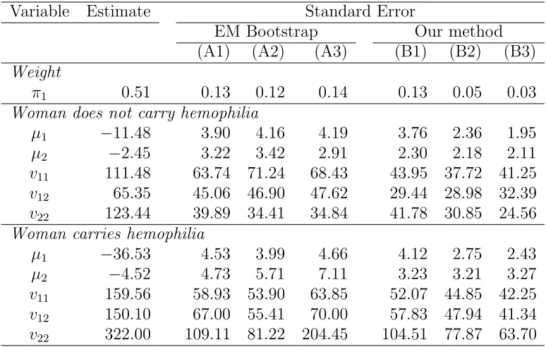
The hemophilia data were collected by Habbema et al. (1974), and were extensively analyzed in a number of papers; see inter alia McLachlan and Peel (2000, pp. 103–104). The question is how to discriminate between ‘nor-mal’ women and hemophilia A carriers on the basis of measurements on two variables: antihemophilic factor (AHF) activity and AHF-like antigen. We have 30 observations on women who do not carry the hemophilia gene and 45 observations on women who do carry the gene. We thus have n = 75 observations on m= 2 features from g = 2 groups of women.
Table 1: Estimation results—Hemophilia data Variable Estimate Standard Error
EM Bootstrap Our method (A1) (A2) (A3) (B1) (B2) (B3)
Weight
π1 0.51 0.13 0.12 0.14 0.13 0.05 0.03
Woman does not carry hemophilia
µ1 −11.48 3.90 4.16 4.19 3.76 2.36 1.95
µ2 −2.45 3.22 3.42 2.91 2.30 2.18 2.11
v11 111.48 63.74 71.24 68.43 43.95 37.72 41.25
v12 65.35 45.06 46.90 47.62 29.44 28.98 32.39
v22 123.44 39.89 34.41 34.84 41.78 30.85 24.56
Woman carries hemophilia
µ1 −36.53 4.53 3.99 4.66 4.12 2.75 2.43
µ2 −4.52 4.73 5.71 7.11 3.23 3.21 3.27
v11 159.56 58.93 53.90 63.85 52.07 44.85 42.25
v12 150.10 67.00 55.41 70.00 57.83 47.94 41.34
v22 322.00 109.11 81.22 204.45 104.51 77.87 63.70
errors (except for π1) have been multiplied by 100 to facilitate presentation.
The EM bootstrap results are obtained from 100 samples for each method and the standard errors correspond closely to those reported in the literature. The three EM bootstraps standard errors are roughly of the same order of magnitude. We shall compare our information-based standard errors with the parametric bootstrap (A1), which is the most relevant here given our focus on multivariate normal mixtures.
The standard errors obtained by the explicit score and Hessian formulae are somewhat smaller than the bootstrap standard errors, which confirms the finding in Basford et al. (1997) concerning I−1
1 (outer score). In eight
of the eleven cases, the standard errors computed fromI−1
2 (Hessian) lie
in-between the standard error based on the score and the standard error based on the robust estimator, as predicted in Section 3. When this happens, the misspecification-robust standard error (B3) is the smallest of the three. For both groups of women the robust standard error is about 63% of the stan-dard error based on parametric bootstrap (A1).
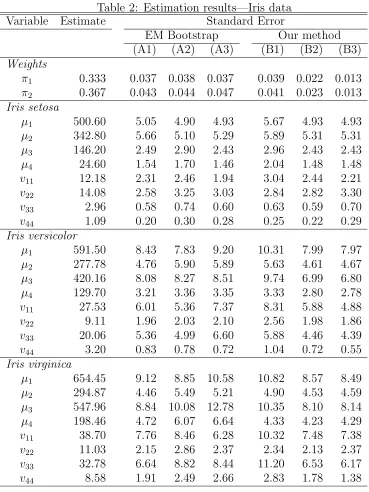
The Iris data set
located on the eastern tip of the province of Qu´ebec in Canada. The data set consists of fifty samples from each of three species of Iris flowers: Iris setosa (Arctic iris), Iris versicolor (Southern blue flag), and Iris virginica (Northern blue flag). Four features were measured from each flower: sepal length, sepal width, petal length, and petal width. Based on the combination of the four features, Sir Ronald Fisher (1936) developed a linear discriminant model to determine which species they are.
The data set thus consists of n = 150 measurements on m = 4 features from g = 3 Iris species. Table 2 contains parameter estimates and standard errors of the means µi and variances vii (the covariance estimates vij for
i 6= j have been omitted), where all estimates and standard errors (except
π1 and π2) have again been multiplied by 100. As before, the EM bootstrap
results are obtained from 100 samples for each method and the standard errors correspond closely to those reported in the literature.
In contrast to the first example, the standard errors obtained by I−1
1
(outer score) are somewhat larger than the parametric bootstrap standard errors, again in accordance to the finding in Basford et al. (1997). In 18 of the 26 cases, the standard errors computed fromI−1
2 (Hessian) lie in-between
the standard error based on the score and the standard error based on the robust estimator, as predicted in Section 3. And again, remarkably, when this happens the misspecification-robust standard error (B3) is the smallest of the three. In this example, contrary to the previous example, the robust standard error is only slightly smaller on average than the standard error based on parametric bootstrap.
Our two examples demonstrate that the implementation of second-order derivative formulae is a practical alternative to the currently used bootstrap. Our program for computing the standard errors ofI−1
1 (outer product),I
−1
2
(Hessian), and I−1
3 (sandwich) is extremely fast. The resulting standard
errors are comparable in size to the bootstrap standard errors, but they are sufficiently different to justify the question which standard errors are the most accurate. This question can not be answered in estimation exercises. We need a small Monte Carlo experiment where the precision of the estimates is known.
7
Simulations
Table 2: Estimation results—Iris data Variable Estimate Standard Error
EM Bootstrap Our method (A1) (A2) (A3) (B1) (B2) (B3)
Weights
π1 0.333 0.037 0.038 0.037 0.039 0.022 0.013
π2 0.367 0.043 0.044 0.047 0.041 0.023 0.013
Iris setosa
µ1 500.60 5.05 4.90 4.93 5.67 4.93 4.93
µ2 342.80 5.66 5.10 5.29 5.89 5.31 5.31
µ3 146.20 2.49 2.90 2.43 2.96 2.43 2.43
µ4 24.60 1.54 1.70 1.46 2.04 1.48 1.48
v11 12.18 2.31 2.46 1.94 3.04 2.44 2.21
v22 14.08 2.58 3.25 3.03 2.84 2.82 3.30
v33 2.96 0.58 0.74 0.60 0.63 0.59 0.70
v44 1.09 0.20 0.30 0.28 0.25 0.22 0.29
Iris versicolor
µ1 591.50 8.43 7.83 9.20 10.31 7.99 7.97
µ2 277.78 4.76 5.90 5.89 5.63 4.61 4.67
µ3 420.16 8.08 8.27 8.51 9.74 6.99 6.80
µ4 129.70 3.21 3.36 3.35 3.33 2.80 2.78
v11 27.53 6.01 5.36 7.37 8.31 5.88 4.88
v22 9.11 1.96 2.03 2.10 2.56 1.98 1.86
v33 20.06 5.36 4.99 6.60 5.88 4.46 4.39
v44 3.20 0.83 0.78 0.72 1.04 0.72 0.55
Iris virginica
µ1 654.45 9.12 8.85 10.58 10.82 8.57 8.49
µ2 294.87 4.46 5.49 5.21 4.90 4.53 4.59
µ3 547.96 8.84 10.08 12.78 10.35 8.10 8.14
µ4 198.46 4.72 6.07 6.64 4.33 4.23 4.29
v11 38.70 7.76 8.46 6.28 10.32 7.48 7.38
v22 11.03 2.15 2.86 2.37 2.34 2.13 2.37
v33 32.78 6.64 8.82 8.44 11.20 6.53 6.17
construct matrices Ai such thatAiA
′
i =Vi. We then obtainRsamples, each of size n, from this distribution where each sample is generated as follows.
• Draw a sample of size n from the categorical distribution defined by Pr(z =i) =πi. This gives n integer numbers, say z1, . . . , zn, such that
1≤zj ≤g for all j.
• Define ni as the number of times that zj =i. Notice that Pini =n.
• For i = 1, . . . , g draw mni standard-normal random numbers and as-semble these in m×1 vectors ǫi,1, . . . ,ǫi,ni. Now define
xi,ν =µi+Aiǫi,ν ∼N(µi,Vi) (ν = 1, . . . , ni).
The set {xi,ν} then consists of n m-dimensional vectors from the required mixture. Given this sample of sizenwe estimate the parameters and standard errors, assuming that we know the distribution is a mixture of g normals.
We perform R replications of this procedure. For each r = 1, . . . , R
we obtain an estimate of each of the parameters. The R estimates together define a distribution for each parameter estimate, and ifRis sufficiently large the variance of this distribution is the ‘true’ variance of the estimator. Our question now is how well the information-based standard error approximate this ‘true’ standard error. We perform four experiments. In each case we take m=g = 2,π1 =π2 = 0.5, and we letn = 100 andn = 500 respectively.
(a) Correct specification. The mixture distributions are both normal. There is no misspecification, so the model is the same as the data-generating process. We let
µ1=
0 0
, µ2 =
5 5
, V1 =
1 0 0 1
, V2 =
2 1 1 2
.
(b) Overspecification. Same as (a), except that
V1 =V2=
1 0 0 1
.
However, we do not know that the variance matrices are the same and hence we estimate them separately.
(d) Misspecification in distribution. The two mixture distributions are not normal. The true underlying distributions areF(k1, k2), but we are
ignorant about this and take them to be normal. Instead of sampling from a multivariate F-distribution we draw a sample {η∗
h} from the univariate F(k1, k2)-distribution. We then define
ηh = s
k1(k2−4)
2(k1+k2−2)
k2−2
k2
η∗
h−1
,
so that the{ηh}are independent and identically distributed with mean zero and variance one, but of course there will be skewness and kurtosis. For i = 1, . . . , g draw mni random numbers ηh in this way, assemble these in m×1 vectors ǫi,1, . . . ,ǫi,ni, and obtain xi,ν as before. We let k1 = 5 and k2 = 10, so that the first four moments exist but the fifth
and higher moments do not.
Each estimation method provides an algorithm for obtaining estimates and standard errors of the parameters θj, which we denote as ˆθj and sj =
c
var1/2(ˆθj) respectively. Based onRreplications we approximate the distribu-tions of ˆθj and sj from which we can compute moments of interest. Letting
ˆ
θj(r)ands(jr)denote the estimates in ther-th replication, we find the standard error (SE) of ˆθj as
SE(ˆθj) = v u u t1
R
R X
r=1
(ˆθj(r)−θ¯j)2, θ¯
j = 1
R
R X
r=1
ˆ
θ(jr).
We wish to know whether the reported standard errors are close to the actual standard errors of the estimators, and we evaluate this ‘closeness’ in terms of the root mean squared error (RMSE) of the standard errors of the parameter estimates. We first compute
S1j = 1
R
R X
r=1
s(jr), S2j = 1
R
R X
r=1
(s(jr))2,
from which we obtain
SE(sj) =qS2j−S12j.
In order to find the bias and mean squared error of sj we need to know the ‘true’ value of sj. For sufficiently largeR, this value is given by SE(ˆθj). We find
BIAS(sj) =S1j−SE(ˆθj), RMSE(sj) = q
and thus we obtain the RMSE, BIAS, and SE of sj for each j.
In our experiments we use R = 50,000 replications for computing the ‘true’ standard errors (10,000 in case (d)) and R = 10,000 replications for computing the estimated standard errors (1000 in case (d)). The reason we use less replications in case (d) is that we want to avoid draws with badly sep-arated means that could induce label switching. To compute bootstrap-based standard errors, we rely on 100 bootstrap samples (Efron and Tibshirani 1993). We use the EMMIX Fortran code converted to run in R to generate mixture samples, and obtain parameter estimates and bootstrap-based stan-dard errors. We then import the parameter estimates into MATLAB and use them to obtain the information-based standard error estimates.
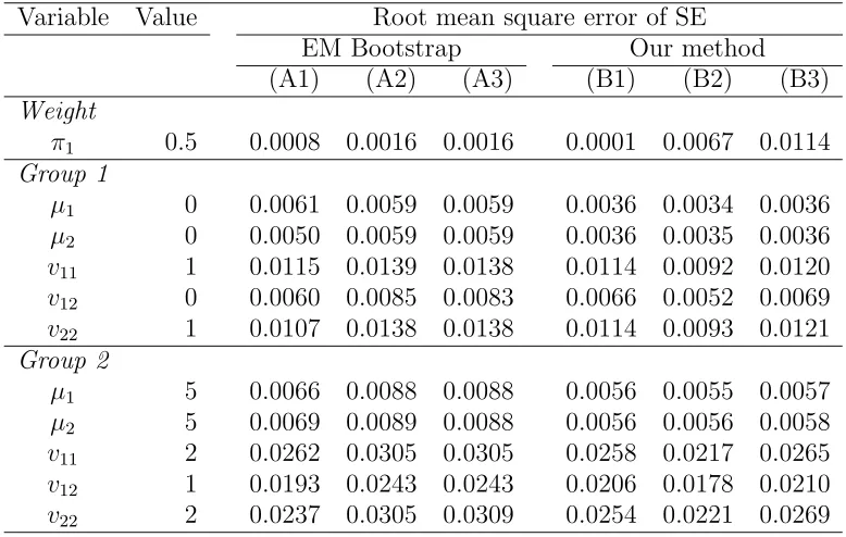
[image:18.595.101.490.451.698.2]Notice that in all four cases the means are well separated. This is use-ful for three reasons: first, label switching problems across simulations are less likely to occur; second, the ML estimates for well-separated means are accurate enough to allow us to focus on standard error analysis rather than in-accuracies in parameter estimates; and third, we expect the bootstrap-based standard errors to work particularly well when accurate parameter estimates are used for bootstrap samples. Thus, to bring out possible advantages of the information-based method, we consider cases where the bootstrap-based methods should work particularly well.
Table 3: Simulation results, case (a), n= 500 Variable Value Root mean square error of SE
EM Bootstrap Our method (A1) (A2) (A3) (B1) (B2) (B3)
Weight
π1 0.5 0.0008 0.0016 0.0016 0.0001 0.0067 0.0114
Group 1
µ1 0 0.0061 0.0059 0.0059 0.0036 0.0034 0.0036
µ2 0 0.0050 0.0059 0.0059 0.0036 0.0035 0.0036
v11 1 0.0115 0.0139 0.0138 0.0114 0.0092 0.0120
v12 0 0.0060 0.0085 0.0083 0.0066 0.0052 0.0069
v22 1 0.0107 0.0138 0.0138 0.0114 0.0093 0.0121
Group 2
µ1 5 0.0066 0.0088 0.0088 0.0056 0.0055 0.0057
µ2 5 0.0069 0.0089 0.0088 0.0056 0.0056 0.0058
v11 2 0.0262 0.0305 0.0305 0.0258 0.0217 0.0265
v12 1 0.0193 0.0243 0.0243 0.0206 0.0178 0.0210
Let us now discuss the simulation results, where we confine our discus-sion to the standard errors of the ML estimates, because the ML estimates themselves are the same for each method. In Table 3 we report the RMSE of the estimated standard errors forn = 500 in the correctly specified case (a). We see that method (B2) based on I−1
2 (the Hessian) outperforms the EM
parametric bootstrap method (A1), which in turn is slightly better than methods (B3) (sandwich) and (B1) (outer score). The observed information matrixI−1
1 based on the outer product of the scores typically performs worst
of the three information-based estimates and is therefore not recommended. The poor performance of the outer score matrix confirms results in previous studies, see for example Basford et al. (1997). In correctly specified cases we would expect that the parametric bootstrap and the Hessian-based ob-served information matrix perform well relative to other methods, and this is indeed the case. Our general conclusion for correctly specified cases is that method (B2) based on I−1
2 performs best, followed by the parametric
bootstrap method (A1). In contrast to the claim of Day (1969) and McLach-lan and Peel (2000, p. 68) that one needs very large sample sizes before the observed information matrix gives accurate results, we find that very good accuracy can be obtained for n = 500 and even forn = 100.
The mean squared error of the standard error is the sum of the variance and the square of the bias. The contribution of the bias is small. In the case reported in Table 3, the ratio of the absolute bias to the RMSE is 9% for method (B2) when we average over all 11 parameters. The bias is typically negative for all methods. As McLachlan and Peel (2000, p. 67) point out, delta methods such as the ‘supplemented’ EM method or the conditional bootstrap often underestimate the standard errors, and the same occurs here. Since the bias is small in all correctly specified models, this is not a serious problem.
We notice that the RMSE of the standard error of the mixing proportion ˆ
π1 is relatively high for methods (B2) and (B3), both of which employ the
Hessian matrix. The situation is somewhat different here than for the other parameters, because the standard error of ˆπ1 is estimated very precisely but
with a relatively large negative bias. Of course, the bias decreases when n
increases, but in small samples the standard error of ˆπ1 is systematically
underestimated. This seems to be a general phenomenon when estimating mixing proportions with information-based methods, and it can possibly be repaired through a bias-correction factor. We do not, however, pursue this problem here. Even with the relatively large RMSE of the mixing proportion, method (B2) performs best, and this underlines the fact that this method estimates the standard errors of the means µi and the variance components
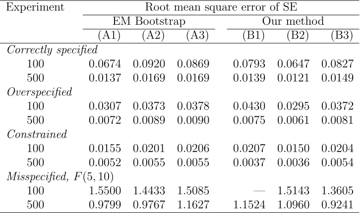
Table 4: Overview of the four simulation experiments Experiment Root mean square error of SE
EM Bootstrap Our method (A1) (A2) (A3) (B1) (B2) (B3)
Correctly specified
100 0.0674 0.0920 0.0869 0.0793 0.0647 0.0827 500 0.0137 0.0169 0.0169 0.0139 0.0121 0.0149
Overspecified
100 0.0307 0.0373 0.0378 0.0430 0.0295 0.0372 500 0.0072 0.0089 0.0090 0.0075 0.0061 0.0081
Constrained
100 0.0155 0.0201 0.0206 0.0207 0.0150 0.0204 500 0.0052 0.0055 0.0055 0.0037 0.0036 0.0054
Misspecified, F(5,10)
100 1.5500 1.4433 1.5085 — 1.5143 1.3605 500 0.9799 0.9767 1.1627 1.1524 1.0960 0.9241
In Table 4 we provide a general overview of the RMSE results of all four cases considered, forn = 100 andn= 500. In cases (b) and (c) we illustrate the special case where V1 =V2. In case (b) we are ignorant of this fact and
hence the model is overspecified but not misspecified. In case (c) we take the constraint into account and this leads to more precision of the standard errors. The RMSE is reduced by about 50% when n = 100 and by about 35% when n = 500. Again, the Hessian-based estimate I−1
2 is the most
accurate of the six variance matrix estimates considered. In case (d) we consider misspecified models where both skewness and kurtosis are present in the underlying distributions, but ignored in the estimation. One would expect that the nonparametric bootstrap estimates (A2) and (A3) and our proposed sandwich estimate (B3) would perform well in misspecified models, and this is usually, but not always, the case. Our sandwich estimate I−1
3 has
the lowest RMSE in all cases. The outer score estimate (B1) fails to produce credible outcomes whenn = 100. If we repeat the experiment based on other
F-distributions we obtain similar results.
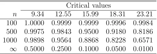
Finally we consider the information matrix test presented in Section 4. The IM test has limitations in practice because the asymptoticχ2-distribution
gm(m+ 3)/2 = 10 degrees of freedom. In Table 5 we compute the sizes for
Table 5: Size of IM test, simulation results Critical values
n 9.34 12.55 15.99 18.31 23.21 100 1.0000 0.9999 0.9999 0.9996 0.9984 500 0.9975 0.9843 0.9500 0.9180 0.8186 1000 0.9898 0.9564 0.8868 0.8228 0.6571
∞ 0.5000 0.2500 0.1000 0.0500 0.0100
n = 100, 500, and 1000, based on 10,000 replications and using the criti-cal values that are valid in the asymptotic distribution. As expected, the results are not encouraging, thus confirming findings by many authors; see Davidson and MacKinnon (2004, Sec. 16.9). There is, however, a viable al-ternative based on the same IM statistic, proposed by Horowitz (1994) (see also Davidson and MacKinnon 2004, pp. 663–665), namely to bootstrap the critical values of the IM test for each particular application. This is what we recommend.
8
Conclusions
Despite McLachlan and Krishnan’s (1997, p. 111) claim that analytical deriva-tion of the Hessian matrix of the loglikelihood for multivariate mixtures seems to be difficult or at least tedious, we show that it pays to have these formu-lae available for normal mixtures. In correctly specified models the method based on the observed Hessian-based information matrix I−1
2 is the best in
terms of RMSE. In misspecified models the method based on the sandwich matrixI−1
3 is the best, even if the standard errors of the observed information
matrix based on the outer product of the scores are large, as is sometimes the case. In general, the bias of the two methods is either the smallest in their category (correctly specified or misspecified) or if not, it becomes the smallest as the sample size increases to n = 500. Our MATLAB code for computing the standard errors runs in virtually no time unless both m and
g are very large, and it is even faster than the bootstrap.
There are at least two additional advantages in using information-based methods. First, the Hessian we computed can be useful to detect instances where the EM algorithm has not converged to the ML solution. Second, if the sample size is not too large relative to the number of parameters to estimate, the methods based on I−1
2 and I
−1
3 can be readily used to compute
intervals are often difficult to compute.
Appendix: Proofs
Proof of Theorem 1. Let φit and αit be defined as in (5). Then, since
f(xt) =Piφit, we obtain
dlogf(xt) = df(xt)
f(xt) = g X i=1 dφit P
jφjt =
g X
i=1
αitdlogφit (10)
and
d2logf(xt) = d
2f(xt)
f(xt) −
df(xt)
f(xt) 2!
=
P
id2φit P
jφjt
−
P idφit P
jφjt !2
= g X
i=1
αit(d2logφit+ (dlogφit)2)−( g X
i=1
αitdlogφit)2 !
. (11)
To evaluate these expressions, we need the first- and second-order derivatives of logφit. Since, using (2),
logfi(x) =−
m
2 log(2π)− 1
2log|Vi| − 1
2(x−µi)
′ V−1
i (x−µi),
we find
dlogfi(x) =−1
2dlog|Vi|+ (x−µi)
′ V−1
i dµi− 1
2(x−µi)
′ d(V−1
i )(x−µi)
=−1
2tr(V
−1
i dVi) + (x−µi)
′ V−1
i dµi+ 1
2(x−µi)
′ V−1
i (dVi)V
−1
i (x−µi)
and
d2logfi(x) = − 1
2tr (dV
−1
i )dVi
−(dµi)′ V−1
i (dµi) + (x−µi)′
(dV−1
i )dµi−(x−µi)′Vi−1(dVi)V
−1
i dµi
−(x−µi)′ V−1
i (dVi)V
−1
i (dVi)V
−1
i (x−µi) = 1
2trV
−1
i (dVi)V
−1
i dVi−(dµi)
′ V−1
i (dµi)
−2(x−µi)′ V−1
i (dVi)V
−1
i dµi
−(x−µi)′ V−1
i (dVi)V
−1
i (dVi)V
−1
and hence, using (3) and the definitions (6)–(8),
dlogφit =dlogπi+ (xt−µi)′Vi−1dµi− 1 2trV
−1
i dVi
+1
2(xt−µi)
′ V−1
i (dVi)V
−1
i (xt−µi)
=a′
idπ+b
′
itdµi− 1
2tr (BitdVi) =a′
idπ+b
′
itdµi− 1
2(vecBit)
′
DdvechVi
=a′
idπ+c
′
itdθi (12)
and
d2logφit=d2logπi−(dµi)
′ V−1
i (dµi)−2(xt−µi)
′ V−1
i (dVi)V
−1
i (dµi)
−(xt−µi)
′ V−1
i (dVi)V
−1
i (dVi)V
−1
i (xt−µi) +1
2trV
−1
i (dVi)V
−1
i (dVi) =−(dπ)′
aia′
i(dπ)−(dµi)
′ V−1
i (dµi)−2b
′
it(dVi)V
−1
i (dµi)
−1
2tr(V
−1
i −2Bit)(dVi)V
−1
i (dVi) =−(dπ)′
aia′
i(dπ)−(dµi)
′ V−1
i (dµi)−2(dvecVi)
′
(bit⊗Vi−1)(dµi)
−1
2(dvecVi)
′
((V−1
i −2Bit)⊗V
−1
i )(dvecVi) =−(dπ)′
aia′
i(dπ)−(dµi)
′ V−1
i (dµi)−2(dvechVi)
′ D′
(bit⊗V
−1
i )(dµi)
−1
2(dvechVi)
′ D′
((V−1
i −2Bit)⊗V
−1
i )D(dvechVi)
=−
dπ dθi
′ aia′
i 0
0 Cit
dπ dθi
. (13)
Inserting (12) in (10), and (12) and (13) in (11) completes the proof.
Proof of Theorem 2. This follows from the expression of Wt(θ) and the development in Lancaster (1984).
Proof of Theorem 3. From (12) we see that
dlogφit =a′idπ+c
′
itdθi =a′idπ+b
′
itdµi− 1
2(vecBit)
and from (13) that
d2logφit=−(dπ)
′ aia′
i(dπ)−(dθi)
′
Cit(dθi) =−(dπ)′
aia′
i(dπ)−(dµi)
′ V−1
(dµi)−2(dµi)
′
(b′
it⊗V
−1
)D(dv)
− 1
2(dv)
′ D′
((2bitb′
it−V
−1
)⊗V−1
)D(dv).
The results then follow—after some tedious but straightforward algebra—
from (10) and (11).
References
Aitken, M., and Rubin, D. B. (1985), “Estimation and Hypothesis Testing in Finite Mixture Models,” Journal of the Royal Statistical Society, Ser. B, 47, 67–75.
Ali, M. M., and Nadarajah, S. (2007), “Information Matrices for Normal and Laplace Mixtures,” Information Sciences, 177, 947–955.
Anderson, E. (1935), “The Irises of the Gasp´e Peninsula,” Bulletin of the American Iris Society, 59, 2-5.
Basford, K. E., Greenway, D. R., McLachlan, G. J., and Peel, D. (1997), “Standard Errors of Fitted Means Under Normal Mixture Models,”
Computational Statistics, 12, 1–17.
Behboodian, J. (1972), “Information Matrix for a Mixture of Two Normal Distributions,” Journal of Statistical Computation and Simulation, 1, 1–16.
Chesher, A. D. (1983), “The Information Matrix Test: Simplified Calcula-tion via a Score Test InterpretaCalcula-tion,” Economics Letters, 13, 15–48.
Davidson, R., and MacKinnon, J. G. (2004),Econometric Theory and Meth-ods, New York: Oxford University Press.
Day, N. E. (1969), “Estimating the Components of a Mixture of Normal Distributions,” Biometrika, 56, 463–474.
Dempster, A. P., Laird, N. M., and Rubin, D. B. (1977), “Maximum Likeli-hood from Incomplete Data via the EM Algorithm” (with discussion),
Dietz, E., and B¨ohning, D. (1996), “Statistical Inference Based on a Gen-eral Model of Unobserved Heterogeneity,” in Advances in GLIM and Statistical Modeling, eds. L. Fahrmeir, F. Francis, R. Gilchrist, and G. Tutz, Lecture Notes in Statistics, Berlin: Springer, pp. 75-82.
Efron, B. (1979), “Bootstrap Methods: Another Look at the Jackknife,”
The Annals of Statistics, 7, 1-26.
Efron, B., and Tibshirani, R. (1993), An Introduction to the Bootstrap, London: Chapman & Hall.
Fisher, R. A. (1936), “The Use of Multiple Measurements in Taxonomic Problems,” Annals of Eugenics, 7, 179–188.
Habbema, J. D. F., Hermans, J., and van den Broek, K. (1974), “A Step-Wise Discriminant Analysis Program Using Density Estimation,” in
Proceedings in Computational Statistics, Compstat 1974, Wien: Phys-ica Verlag, pp. 101–110.
Hathaway, R. J. (1985), “A Constrained Formulation of Maximum-Likelihood Estimation for Normal Mixture Distributions,” The Annals of Statis-tics, 13, 795–800.
Horowitz, J. L. (1994), “Bootstrap-Based Critical Values for the Information Matrix Test,” Journal of Econometrics, 61, 395–411.
Huber, P. J. (1967), “The Behavior of Maximum Likelihood Estimates un-der Non-Standard Conditions,” in Proceedings of the Fifth Berkeley Symposium on Mathematical Statistics and Probability, Vol. 1, eds. L. M. LeCam and J. Neyman, Berkeley: University of California Press, pp. 221–233.
Lancaster, A. (1984), “The Covariance Matrix of the Information Matrix Test,” Econometrica, 52, 1051–1053.
Liu, C. (1998), “Information Matrix Computation from Conditional Infor-mation via Normal ApproxiInfor-mation,” Biometrika, 85, 973–979.
Louis, T. A. (1982), “Finding the Observed Information Matrix When Using the EM Algorithm,”Journal of the Royal Statistical Society, Ser. B, 44, 226–233.
Magnus, J. R., and Neudecker, H. (1988),Matrix Differential Calculus with Applications in Statistics and Econometrics, Chichester/New York: John Wiley, Second edition, 1999.
McLachlan, G. J., and Basford, K.E. (1988),Mixture Models: Inference and Applications to Clustering, New York: Marcel Dekker.
McLachlan, G. J., and Krishnan, T. (1997), The EM Algorithm and Exten-sions, New York: John Wiley.
McLachlan, G. J., and Peel, D. (2000), Finite Mixture Models, New York: John Wiley.
McLachlan, G. J., Peel, D., Basford, K. E., and Adams, P. (1999), “Fitting of Mixtures of Normal and t-Components,” Journal of Statistical Soft-ware, 4, Issue 2, www.maths.uq.edu.au/∼gjm/emmix/emmix.html.
Newton, M. A., and Raftery, A. E. (1994), “Approximate Bayesian Inference with the Weighted Likelihood Bootstrap” (with discussion), Journal of the Royal Statistical Society, Ser. B, 56, 3–48.
Newcomb, S. (1886), “A Generalized Theory of the Combination of Obser-vations so as to Obtain the Best Result,” American Journal of Mathe-matics, 8, 343–366.
Pearson, K. (1894), “Contribution to the Mathematical Theory of Evo-lution,” Philosophical Transactions of the Royal Society, Ser. A, 185, 71–110.
Stigler, S. M. (1986), The History of Statistics: The Measurement of Un-certainty Before 1900, Cambridge, MA: Belknap.
Titterington, D. M., Smith, A. F. M., and Makov, U. E. (1985),Statistical Analysis of Finite Mixture Distributions, New York: John Wiley.
White, H. (1982), “Maximum Likelihood Estimation of Misspecified Mod-els,” Econometrica, 50, 1–26.