http://dx.doi.org/10.4236/jcc.2016.45008
Exploring the Big Data Using a Rigorous and
Quantitative Causality Analysis
X. San Liang
School of Marine Sciences and School of Mathematics, Nanjing University of Information Science and Technology, Nanjing, China
Received 28 April 2016; accepted 19 May 2016; published 26 May 2016
Abstract
Causal analysis is a powerful tool to unravel the data complexity and hence provide clues to achieving, say, better platform design, efficient interoperability and service management, etc. Data science will surely benefit from the advancement in this field. Here we introduce into this commu-nity a recent finding in physics on causality and the subsequent rigorous and quantitative causali-ty analysis. The resulting formula is concise in form, involving only the common statistics namely sample covariance. A corollary is that causation implies correlation, but not vice versa, resolving the long-standing philosophical debate over correlation versus causation. The applicability to big data analysis is validated with time series purportedly generated with hidden processes. As a demonstration, a preliminary application to the gross domestic product (GDP) data of United States, China, and Japan reveals some subtle USA-China-Japan relations in certain periods.
Keywords
Causality, Big Data, Information Flow, Time Series, Causal Network
1. Introduction
We have entered an era of data wealth; how to analyze these data has become a big problem for scientists in the twenty-first century. This raises many challenging issues, among which is causal inference, a field which ac-tually forms an important subject in many different scientific disciplines, even in philosophy (e.g., [1]). For data science, it will help to unravel the complexity of the ever-growing datasets, and hence help to build platforms for efficient management and better service.
Causality analysis, however, is a very challenging problem. In their book Doing Data Science (p. 274) [2], O’Neil and Schutt remarked, “One of the biggest statistical challenges, from both a theoretical and practical perspective, is establishing a causal relationship between two variables.” In the past few years, there has been a surge of interest in this field, echoing the call from the newly emerged science of big data. Many empirical or half-empirical formalisms have been proposed, and they generally work well in their specific contexts (see the references in [3]).
hy-55
pothesis testing (e.g., [5]), is actually a problem in physics; causality is actually a real physical notion, which can be put on a rigorous footing. With the Liang14 formalism, many problems, which traditional approaches fail to handle, turn out to be easy. It also unambiguously and explicitly resolves the long-standing debate in philosophy regarding correlation versus causation, and has been successfully applied to many real world problems.
However, this line of work has not even been touched in big data studies. While we should avail ourselves of the arsenal of traditional tools, new ideas, particularly new ideas like this one which is based firmly on physical footing, will for sure facilitate the advancement of the new science. We are therefore motivated to introduce the newly developed causality analysis to data scientists. This makes the main purpose of this study.
In the following we first give a brief review of the formalism, its development and major results. To test its utility in handling big data, in Section 3 we purportedly generate series in extreme situations, particularly series in the presence of hidden processes. As a demonstration, Section 4 presents a preliminary application to the study of the USA-China-Japan relation. This study is summarized in Section 4.
2. Theoretical Development and Applications
Historically Granger [5] formulated causality analysis as a statistical hypothesis test, which has now been re-ferred to as Granger causality analysis. On the other hand, another real physical notion, namely, information flow, or information transfer as it may appear in the literature, has been developed for over three decades. In-formation flow has applications in a wide variety of disciplines; people gradually realize that central at the field, which makes it widely applicable, turns out to be its logical association to causality. This observation has further been substantiated as it was established that Granger causality and the most popular empirical measure of in-formation flow so far, namely, transfer entropy [6], is actually equivalent [7].
So the two major lines of work on causality analysis eventually merge. The corresponding formalisms, how-ever, have long been found unable to verify themselves in many applications, or they may even yield spurious causal relations. The verification is based on the following observation:
If the evolution of a variable, say, X1, is independent of another one, X2, then the causality from X2 to X1
vanishes.
Hereafter we will call it Principle of Nil Causality. Recently, Smirnov [8] gave this a systematic investigation, and concluded that they cannot verify the principle in a wide range of situations; similar results also show in [9]. In response to the call from the new science of big data, we should touch the base and re-examine the problem carefully.
Since causality can be quantitatively measured by information flow, while information flow is a real physical notion (not just something in statistics), Liang argued that it should be formulated on a rigorous footing, rather than be proposed as an ansatz [3] [10]. Besides, the above principle should be stated as a proven theorem, not something to be verified in applications. In this spirit, Liang [10] considered a stochastic system in the form
(
)
1 1 1, 2, 11 1 12 2,
dX =F X X t dt b dW+ +b dW (1)
(
)
2 2 1, 2, 21 1 22 2,
dX =F X X t dt b dW+ +b dW (2)
where (W1, W2) is a vector of standard Wiener process, and F1 and F2 are differentiable functions of (X1, X2). He
obtained the following theorems: Theorem 2.1. (Liang, 2008)
For the dynamical system (1)-(2), the rate of information flowing from X2 to X1 is
(
)
(
2 2)
11 12 1 1 1
2 1
1 1 1 2
1 1 1
, 2
b b
F
T E E
x x
ρ ρ
ρ ρ
→
∂ +
∂
= − +
∂ ∂
(3)
where E stands for mathematical expectation, and
ρ
1=ρ
1( )
x1 is the marginal probability density of X1.Theorem 2.2. Principle of nil causality (Liang, 2008)
If in the system (1)-(2), neither F1 nor b11 nor b12 has dependence on X2, then T2→1=0.
If only two time series are given, the information flow between them can be obtained through maximum like-lihood estimation.
Theorem 2.3. (Liang, 2014)
Given two time series X1 and X2, under the assumption of a linear model, the maximum likelihood estimator
(mle) of the rate of information flowing from X2 to X1 is
2 11 12 2, 1 12 1, 1
2 1 2 2
11 22 11 12
.
d d
C C C C C
T
C C C C
→
− =
− (4)
In this equation, C=
( )
Cij is the sample covariance matrix between time series X1 and X2, and Ci dj, thesam-ple covariance between Xi and a series derived from Xj using Euler forward differencing scheme:
(
)
, , 1 ,
j n j n j n
X = X + −X ∆t.
Note in (4) the T is actually the mle of the information flow, and, strictly, should bear a hat. We abuse the no-tation here as, from now on, only (4) will be used, and hence no confusion will arise. That is to say, (4) will be taken as the quantitative measure of causality from X2 to X1. More precisely, the absolute value of T measures
the causality. When T2→1 >0, X2 is causal to X1; if T2→1=0, X2 is not the cause of X1.
The formula for information flow hence causality is very concise. Considering that in history there is a long-standing debate over correlation versus causation, one may transform it into a form in terms of correlation coefficient:
(
)
2 1 2 2, 1 1, 1 ,
1 d d
r
T r rr
r
→ = − ′ − ′ (5)
with 12
11 22
C r
C C
= the correlation coefficient, and i dj, i dj, .
ii jj
C r
C C
′ = Observe that, if r=0, then T2→1=0; but
if T2→1=0, r does not necessarily vanish. Contrapositively, this means that
Causation implies correlation, but correlation does not imply causation.
Causality can be normalized so as to reveal its relative magnitude; see [4] for details. One may also perform statistical significance test for Equation (4), which is referred to [3].
Equation (4) has been validated with touchstone problems that fail the traditional Granger causality analysis. It has also been applied to many real world problems, with remarkable success. Among these applications is the causal structure study between CO2 and global warming [11]. It is found that the CO2 concentration rise during
the past 120 years does cause the recent global warming; the causal relation is one-way, i.e., from CO2 to global
atmosphere temperature. However, on a 1000-year (or over) scale, the causality is totally reversed; i.e., it is global warming that causes CO2 to increase, in agreement with that inferred from the ice-core data recently from
Antarctica. Besides, the anthropogenic gas emission mainly from the Northern Hemisphere, however, causes mainly the warming in the Southern Hemisphere.
Another application is with several series of prices of US stocks downloaded from ! finance YAHOO
. Basically each
57
3. Validations
3.1. Validation with Series Generated with a Pair of Processes
Consider the series generated from two autoregressive processes, which traditionally have been used to test cau-sality analysis tools,
( )
0.5(
1)
2(
1)
1 1( )
,X n = X n− +a Y n− +N e n (6)
( )
1(
1)
0.9(
1)
2 2( )
,Y n =b X n− + Y n− +N e n (7)
where e1N
( )
0,1 , e2N( )
0,1 are independent normal processes. First let N1=N2 =1. For different a2 andb1, initialize the system with random numbers between 0 and 1, generate two series with 50000 values, and then
compute the causalities using (4). The results are tabulated in Table 1.
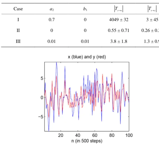
The series generated for case I are shown in Figure 1. By visual inspection they are correlated and look alike. This is not surprising, as Y drives X hence X follows Y. As regards the causalities, since b1=0, Y does not de-pend on X, and hence ideally Tx→y should vanish. Here at a 90% confidence level,
(
4)
3 45 10
x y
T→ = ± × − nats
per iteration, which cannot be viewed as different from zero. In contrast, Ty→x is huge, clearly indicating a one-way causality. This is an example of highly correlated series that results in a zero causality in one direction.
For case II, a2= =b1 0, hence X and Y have nothing to do with each other. A faithful analysis should yield zero causalities for both directions. Indeed, at a 90% level, they can neither be distinguished from zero.
To test the validity of (4), we design a case (case III) with very weak coupling: a2= =b1 0.01. In the equa-tions X and Y are essentially independent, but theoretically there does exist causality, though negligible. Re-markably, our analysis yields two significant causalities, i.e., both of them, albeit very small, pass the signific-ance test.
In order to see whether the negligible causalities can be detected between series immersed in noises, we am-plify e1 and e2 by ten times: N1=N2 =10, and repeat case III. This results in:
(
)
4
11 3 10
y x
T→ = ± × − ,
(
4)
4.7 1.5 10
x y
[image:4.595.169.438.461.706.2]T→ = ± × − , i.e., two information flow rates, albeit negligible, significant at a 90% level, just as one would expect!
Table 1. Absolute information flow rates for the series generated with (6)-(7), and their respective confidence intervals at a 90% significance level. Units are in 10−4 nats per iteration.
Case a2 b1 Ty→x Tx→y
I 0.7 0 4049 ± 32 3 ± 45
II 0 0 0.55 ± 0.71 0.26 ± 0.36
III 0.01 0.01 3.8 ± 1.8 1.3 ± 0.9
58
3.2. Validation with Series in the Presence of a Hidden Process
Our causality analysis is for two time series and, as we showed above, works perfectly for series generated with two processes. However, in real problems, a pair of time series could be the result of a lot of processes, and, moreover, we may have no idea what the processes are, or even are unaware of the existence of those processes. Will (4) still work in this case? In other words, can our analysis work well just the same in the presence of a hidden process? This is a problem where the traditional analyses fail.
Consider a pair of series formed from the X and Y in the following autoregressive processes:
( )
0.5(
1)
2(
1)
0.7(
1)
1 1( )
,X n = X n− +a Y n− + Z n− +N e n (8)
( )
1(
1)
0.9(
1)
0.2(
1)
2 2( )
,Y n =b X n− + Y n− + Z n− +N e n (9)
( )
0.2(
1)
3( )
.Z n = Z n− +e n (10)
Different from (6)-(7), here both X and Y are dependent on a third variable Z.
Pretending that we have no idea about the existence of Z, we perform a causality analysis just as before with the series X and Y. Repeat the experiments in Table 1, and list the computed causalities in Table 2.
The results are just as one would expect. For example, case I is a one-way causal system, and the computed absolute information flow rates confirm this; in case II X and Y are independent, and the calculated causalties are essentially zero in both directions; for case III, the causalities do exist, although they are very small. In a word, our causality analysis is capable of handling the series in the presence of hidden processes, even in extreme cas-es. It then can be utilized for data analysis on a generic basis, and is hence expected to play a role in the new science of big data.
4. A Preliminary Application
As a demonstration, we now take a look at the GDP of USA, China, and Japan, the three economic powers. The data are from World Bank1, available every year from 1960 through 2014. Note it is by no means our intention to conduct a research on international bilateral relation, which requires an in-depth investigation of the related economics and politics and, above all, more reliable data with finer time resolution; we are just about to provide an example to demonstrate how the above new causality analysis tool may allow us to extract the information underlying the data which would be otherwise very difficult, if not impossible, to extract.
Since the GDPs of the three countries soar from 1960 to 2014, we choose to examine their annual growth rates. Shown in Figure 2 are these rates. By visual inspection of the data we can see that the American and Jap-anese GDP growths are highly correlated. But aside from this, it is hard to tell what a structure the three may have. Now our rigorous causality analysis comes to aid.
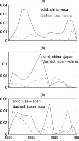
The validation in the preceding section allows us to examine the relations between the three countries regard-less of the GDP data of the rest world, particularly, Europe, though we know the influence of the latter does ex-ist. Since we need to do the covariance estimation, we pick a 40-year window to build the ensemble, and then do a running time estimation. This results in a time period 1980-1995 over which the causalities can be computed. A straightforward application of (4) yields these causalities, which we plot in Figure 3.
First look at Figure 3(a). Because of the small ensemble, most of the values are not significant at a 80% level. But the large ones, particularly some of Tchina→usa are significant. That is to say, during the period, China exerts
more influence on the US economy than US exerts on the Chinese economy. Indeed this makes sense, consider-ing in that period China was not open enough to the western world. Generally this is also the case for Figure 3(b). What makes Figure 3(b) quite different from Figure 3(a) is that, in early 90s’, the influence of Japan on China is large, exceeding the causality in the opposite direction. This does, again, make sense. In early 90s’, the western world imposed strict sanctions against China because of political reasons, but Japan, albeit known as a major western country, did not join them. In that particular period China then had to rely on Japan a lot, result-ing in the dominatresult-ing causality from Japan to China!
For Figure 3(c), the evolutionary pattern is also remarkable. As we said, Japan has a GDP growth history highly correlated to that of USA. What makes the high correlation? We know a one-way causality from one se-ries, say X1, to another, say X2, will result in a correlation, but a causality in the opposite direction, or a mutual
59
Table 2. Absolute information flow rates for the series generated with (8)-(9), and their respective confidence intervals at a 90% significance level. Units are in 10−4 nats per iteration.
Case a2 b1 T2 1→ T1 2→
I 0.7 0 3933 ± 38 22 ± 46
II 0 0 2.9 ± 4.8 2.2 ± 2.4
[image:6.595.229.393.386.677.2]III 0.01 0.01 22 ± 8 19 ± 4
Figure 2. GDP annual growth rates (%) since 1960. Data source: World Bank (http://data.worldbank.org/).
causality, will also make such a correlation. Here the figure shows that the three possibilities all exist in this par-ticular application, nicely spanning different periods (approximately 1980-1987, 1987-1990, 1990-1995). This serves as an excellent example about correlation versus causation, though an explanation of the structure in Figure 3(c) requires more knowledge of the politics and economics in history about the two countries, which we leave to future studies.
5. Summary and Outlook
The emerging data science will for sure benefit from the advancement of other data-related disciplines. In this study, we introduce to the community a recently established rigorous and quantitative causality analysis to help unravel the complexity of big datasets, explore the underlying causal structures, and hence design efficient plat-forms for service and management purposes. To summarize, we here repeat the formula in Theorem 2.3 for causal-ity estimation, that is, for series X1 and X2, the information flow from the latter to the former is estimated to be
2 11 12 2, 1 12 1, 1
2 1 2 2
11 22 11 12
,
d d
C C C C C
T
C C C C
→
− =
−
with Cij the sample covariances between Xi and Xj and Ci dj, that between Xi and a derived series from Xj by taking Euler forward difference. If T2→1 is nonzero, then X2 is causal to X1, and vice versa. An immediate
co-rollary is that causation implies correlation, but correlation does not imply causation.
The above formalism, or Liang14 formalism as referred in the text, has been applied with remarkable success to many real problems. In this study, it has been validated with data series in the presence of hidden processes, and then exemplified with an analysis of the GDP data of USA, China, and Japan. Though the study is prelimi-nary, the result is very encouraging, from an aspect demonstrating its power. This analysis tool is expected to play a role in the new interdisciplinary science, i.e., the science of big data.
Acknowledgements
This study was supported by the National Science Foundation of China under Grant No. 41276032, by Jiangsu Provincial Government through “2015 Jiangsu Program for Innovation Research and Entrepreneurship Groups” and the Jiangsu Chair Professorship, and by the State Oceanic Administration through the Special Program on Global Change and Air-Sea Interaction (GASI-IPOVAI-06).
References
[1] Dempster, A.P. (1990) Causality and Statistics. J. of Statistical Planning & Inference, 25, 261-278. http://dx.doi.org/10.1016/0378-3758(90)90076-7
[2] O’Neil, C. and Schutt, R. (2013) Doing Data Science: Straight Talk from the Frontier. O’Reilly, Cambridge.
[3] Liang, X.S. (2014) Unraveling the Cause-Effect Relation between Time Series. Phys. Rev. E, 90, 052150. http://dx.doi.org/10.1103/PhysRevE.90.052150
[4] Liang, X.S. (2015) Normalizing the Causality between Time Series. Phys. Rev. E, 92, 022126. http://dx.doi.org/10.1103/PhysRevE.92.022126
[5] Granger, C. (1969) Investigating Causal Relations by Econometric Models and Cross-Spectral Methods. Econometrica,
37, 424. http://dx.doi.org/10.2307/1912791
[6] Schreiber, T. (2000) Measuring Information Transfer. Phys. Rev. Lett., 85, 461-464. http://dx.doi.org/10.1103/PhysRevLett.85.461
[7] Barnett, L., Barrett, A.B. and Seth, A.K. (2009) Granger Causality and Transfer Entropy Are Equivalent for Gaussian Variables. Phys. Rev. Lett., 103, 238701. http://dx.doi.org/10.1103/PhysRevLett.103.238701
[8] Smirnov (2013) Spurious Causalities with Transfer Entropy. Phys. Rev. E, 87, 042917.
[9] Lizier, J.T. and Prokopenko, M. (2010) Differentiating Information Transfer and Causal Effect. European Phys. J. B,
73, 605-615. http://dx.doi.org/10.1140/epjb/e2010-00034-5
[10] Liang, X.S. (2008) Information Flow within Stochastic Dynamical Systems. Phys. Rev. E, 78, 031113. http://dx.doi.org/10.1103/PhysRevE.78.031113
[11] Stips, A., Macias, D., Coughlan, C., Garcia-Gorriz, E. and Liang, X.S. (2016) On the Causal Structure between CO2