51
ANALYZE AND EVALUATE THE IMPLEMENTATION
OF
CDS ALGORITHMS USING THE MOBILE AGENT.
.
1RAFAT AHMED ALHANANI, 2JAAFAR ABOUCHABAKA, 3RAFALIA NAJAT
1 2 3 Department of Computer Science, IBN Tofail University, Faculty of Science, Kénitra, Morocco.
E-mail: 1[email protected], 2[email protected], 3arafalia @yahoo.fr
ABSTRACT
In this work, we identify, analysis and evaluate the role of mobile agent to solve the problem of selecting the minimum connected dominating set CDS better alternative approach than the exchange messages approach. The first problem concerns the nature of the CDS construction algorithms in question. Their design is justified as the purpose to construct a virtual infrastructure for wireless network with varied high cost in the permanent exchanged messages to select the CDS. The redundant broadcasting of the packets effects the overall network performance, increases the latency, the collision and the need of synchronization mechanism.
Common techniques and algorithms such as marking process, Greedy Algorithms, Maximal Independent Set MIS, Pruning process, and Multipoint Relaying are exploited to select the potential nodes of the connected dominating set. We analyzed and implemented some of these techniques from the using perspective of the mobile agent.
We shall argue that the mobile agent implements the CDS algorithms with less cost in its moves comparing with the cost of exchanged messages. Mobile agent just requires local information and a limited number of iterative rounds instead of the redundant broadcasting packets that imposed by other techniques. There is no work similar to our work that discusses the using of mobile agent to construct the connected dominating set based on those common techniques.
We have made slight modifications on those algorithms, their notations and parameters to be appropriate through the implementation by the mobile agent. Using the mobile agent shows encouraging results for constructing connected dominating set with few iterations, eliminates the overhead caused by the large volume of message exchange, and improve the structure of the computed CDS. However, the agent by implementing those algorithms successfully constructs the connected dominating set; the constructed connected dominating nodes are still large set. The agent by implementing those algorithms could not construct the minimum CDS.
Keywords- Mobile Agent, Graphic Theory, Connected Dominating set, Maximal Independent Set, Whiteboard.
1. INTRODUCTION
A virtual backbone is a set of selected nodes employed for routing process [2]. The concept of
virtual backbone was first introducedin the literature
[1], as the routing infrastructure of ad hoc networks. Exploiting this concept ensures the reducing of the
exchanged messages, routing-related control
messages and the amount of wireless signal collision and interference from the whole network to the set of backbone nodes. A wireless network lacks a physical infrastructure that manages the nodes and coordinates the exchanged messages among them. Exploiting the virtual backbone overcomes this lack. Thus, any
non-backbone node has to be adjacent to at least one backbone node. Only the nodes in the virtual backbone will be involved in message routing, as a result, the routing protocol will work much faster and efficiently [3]. A virtual backbone plays a significant role in saving energy of limited-energy wireless nodes [4]. More importantly, less involved nodes in message routing, less need to maintain routing information in those nodes. A network can react quickly to changes in the topology [2].
52 constructing this virtual backbone in wireless networks is the Connected Dominating Sets (CDSs) [5]. A subset nodes of a graph G is a dominating set if every node of the graph either belongs to the subset or adjacent to at least one node in the subset. A dominating set is connected, called CDS, if there exists a path only consists of the nodes in the set [6].
The connected dominating set represents as virtual
backbone [9] which is a set D of vertices has two
properties; any node in D can reach any other node
in D by a path that stays entirely within D. That
is, D induces a connected sub-graph of G. Every
node in G either belongs to D or is adjacent to a node
in D. Thus, any non-dominated connected node
wants to communicate will send a packet to one of (one hop away from) the nearest dominated node belongs to the (CDS) connected dominated set which in turn forwards the packet to its destination in efficient way through only the nearest interconnected dominated nodes and takes less number of packet communications and moves. This efficient technique used specially for the wireless ad hoc network, which has no physical backbone infrastructure. Since the networking nodes in wireless ad hoc networks are very limited in resources, a virtual backbone should be low in its number of belonging nodes and be
constructed with low communication and
computation costs.
A minimum connected dominating defined [10] as set of a graph G is a connected dominating set with the smallest possible cardinality among all connected dominating sets of G.
Constructing a CDS based on several techniques and algorithms have raised in literature. The MIS based algorithms usually have good performance bound and time/message complexities. They only need one-hop neighborhood information, but they relies on the single leader or Multiple leader based algorithms. Pruning based algorithms has high message complexity due to the global connectivity checking. The multipoint relaying based heuristic is pure localized. This algorithm selects CDS from a multipoint relay set, but no complexity analysis for this algorithm in literature [7].
Mobile agent is a piece of code with special features such as the ability to sequentially move, clone and run in remote sites in a computer network. It can make decision, search of specific information and gather the results, cooperate, directly communicate through exchanging messages and indirectly through using the whiteboard with other mobile agents and return to its home site after completing the assigned tasks on behalf of its user.
The mobile agent just require the minimum information, as the number of nodes, to explore the network, it does not need to know the whole topology information. The Agent is so convenient for the dynamic environment such wireless networks. Mobile Agent offers the distributed possibility, further the algorithms that based on mobile agent usually have characterized with ease. Ideally, mobile agent just requires local information and a limited number of iterative rounds instead of the redundant broadcasting packets that is imposed by other techniques.
As an initial step and before starting any algorithm to construct CDS, most algorithms depend on exchange routing information among neighbor nodes. The exchange of the required information is based on limited number of hops to ensure the interconnection and the control. The total number of messages is too much and frequently send. That is what can be overcome by using mobile agent. We studded the constructing of CDS algorithms and implemented them using the mobile agent which provides a significant level of flexibility, simplicity. It can be implemented in a number of diverse
domains comparing with CDS traditional
algorithms. For this, when designing a CDS algorithm we take into account besides the stability, the performance bounds, degree of localization, time and message complexities.
In this paper, we focus on various CDS algorithms that have proposed in the literature for constructing CDS as a virtual backbone. As demonstrated that during the implementation of these algorithms, the
nodes exchange their open neighborhood
information with their one-hop neighbors which produce varied high cost in the permanent exchanged messages to select the CDS. The redundant broadcasting of the packets effects the overall network performance, increases the latency, the collision and the energy consumption. The data transmission consumes much energy than data processing. Sending a single bit can consume the same energy as executing 1000 instructions at typical sensor node [30]. Therefore, it will be more energy efficient if the nodes keep its data in its memory and waits for a mobile agent to process and carry the special data.
53 The selected dominating nodes can be used as an optimal itinerary for the mobile agent to reach every node that does not belong to the connected dominating set in order to implement another tasks overall network.
Moreover, after the study and evaluate the CDS algorithms, we implement those evaluated algorithms using the mobile agent. Then, we present how the mobile agent success to construct the connected dominating set, through implementing our evaluated CDS algorithms taking into account minimizing the total number of movements.
Finally, we mentioned that the mobile agent could not select the minimum and optimal CDS even with more constrains and modifications in the implementation procedures of those CDS algorithms.
The rest of the paper organized as follow. In section 2, we discusses the classification of CDS algorithms and elaborates the various algorithms proposed in the literature pertaining to construction of CDS. Section 3 illustrates the used CDS algorithms by the mobile agent and the analytical results. Section 4 concludes the paper.
2. CDS CONSTRUCTION TECHNIQUES
The construction algorithms of the connected dominating set vary on the adopted techniques on which the CDS algorithms have based. Jeremy Blum in [7], P. S. Vinayagam in [8] and Jiguo Yu in [9]
surveyed the exploiting distributed CDS
construction techniques such as: Marking, greedy, MIS based, Steiner tree based, pruning based, and Multipoint Relaying. Those techniques are classified to Centralized and Decentralized algorithms. Algorithms belong to centralized category assume the prior knowledge of network global information. As well as the availability of the complete network topology information, which is usually not practical in the case of mobile wireless networks. While in the Decentralized algorithms, local network information is essential. These algorithms can be further categorized to Distributed and Localized algorithms, [8, 9, 27] for more details.
In this section, we give brief review of some those techniques and their works in order to identify the main differences among them and the most appropriate to be implemented by the mobile agent.
2.1. Based on the Greedy Algorithm
The first technique called the Marking process, which uses different colors to classify the vertices in the graph. The dominating vertex is colored black,
with its neighbor vertices colored gray and other vertices with white color. Two greedy heuristic algorithms for constructing CDS proposed in [10], which guarantees the bounded performance. The first algorithm initially starts by marking all vertices white. Then selects the node with the maximum number of white neighbors, marks it black and marks its white neighbors gray. The algorithm examines the gray nodes simultaneously with their white neighbors. The selected gray node with its white neighbor must have the maximum number of white neighbors. The selected pair of nodes are marked black, with their white neighbors marked gray. The algorithm terminates when all the vertices of the graph are marked gray or black.
The second algorithm starts by marking all vertices white. At the first iteration, it selects a node that reduces the maximum number of a connected black component (the black component is one or more black nodes connect to their gray neighbors). Selected node is marked black and its white neighbors are marked gray. The algorithm does not guarantee the connectedness of the black components. Therefore, in order to connect the black components, a Steiner Tree connects all the black nodes by two or more intermediate gray nodes belong to the two components and change their color to black.
2.2. Based on Maximal Independent Set MIS
A subset nodes of V is an independent set if for
any pair of vertices in V, there is no edge
(connection) between them. A maximal independent
set (MIS) is the independent set in which adding any
extra vertex will cause connection between any pair of nodes in the set. Any maximal independent set is also a dominating set. The technique for constructing the CDS based on MIS can be simultaneously compute and connect the MIS [11] or connect the selected nodes after the construction is over [12, 13, 14], these selected MIS nodes form the skeleton of the CDS, in order to connect the nodes in the MIS, additional nodes are added, thus the CDS is formed. To compute an MIS the algorithm relies on either single leader or multiple leaders, with additional complexity cost. The node has the maximum degree or id among all neighbors can serve as leader.
Cheng et al. propose in [11, 15] their algorithm
54 white nodes to the leader node changed to be a dominatee (gray). A non-active white node changes
to status active if one of its neighbors becomes a
dominate (gray). Its color still keeps white. Then, an active node with the smallest cost among all its active neighbors (the local cost is the id or sometimes a random value with the id) will compete to be a dominator; it then invites its gray parent node to be its dominator. Its minimum cost gray parent also changes to serve as its dominator (black), ensuring the connectivity of the dominating tree. Finally, all black leaf nodes can change back to be dominatees (gray). This process terminates when all nodes are colored gray or black, and all the black nodes form a connected dominating set. This
algorithm has the time complexity of O(n), and the
message complexity of O(n log n), which is
dominated by leader election [7]. As a result, a dominating tree is grown from the leader.
Alzoubi et al. [16] propose an algorithm to
construct the dominating set. They employ the distributed leader election algorithm [17] to construct a rooted spanning tree. With different types of messages used to classify the nodes of the constructed spanning tree, the nodes become either black (dominator) or gray (dominatee), based on their ranks. The rank of a node is the number of hops to the root of the spanning tree with its ID. The labelling process begins from the root node and finishes at the leaves. The node with the lowest rank marks itself black and broadcasts a DOMINATOR message. The marking process then continues according to the following rules:
If the node firstly receives a DOMINATOR
message, it marks itself gray and broadcasts a DOMINATEE message.
If a node received DOMINATEE messages from
all its lower rank neighbors, it marks itself black and sends a dominator message.
Finally, the root node connects the selected nodes of the MIS to form a CDS. It broadcasts an INVITE message. Then, the INVITE message rebroadcasts by dominatee (gray) nodes to all two-hop neighbors out of the current CDS. When a black node receives the INVITE message for the first time, it joins the dominating tree together with the gray node, which broadcasts the message and so on. The process terminates when all the black nodes join the CDS.
This algorithm has time complexity of O(n), and
message complexity of O(n log(n)).
2.3. Based on Pruning CDS Construction
Wu et al.'s work [18, 19] proposes a completely localized algorithm to construct CDS. All the vertices exchange their open neighborhood information with their one-hop neighbors. Thus, each node knows all of its two-hop neighbors. Each node has two unconnected neighbors marks itself as a dominator. The set of marked vertices form a connected dominating set, S, the result is big number of dominator nodes. To avoid the redundant of those nodes, two rules have proposed as follow:
Rule1: a node u deleted from S, the CDS, if there
exists a node v with higher ID such that the closed
neighbor set of u is a subset of the closed neighbor
set of v,(The closed neighbor set of node u is
one-hop neighbors adjacent to u with the node u itself).
Rule2: node u deleted from S when two of its
connected neighbors in S with higher IDs can cover
all of u's neighbors.
Another good pruning-based rule has proposed by Butenko's algorithm in [14, 15]. The connected
dominating set S is initialized to all white nodes of
the graph G, and then each node will be examined to
determine whether it should be still belonging to the
CDS or not. If removing node u from S causes
disconnecting to the induced graph of S, then node u
must be part of the CDS and color it black.
Otherwise, remove ufrom S. At the same time, if u
does not have a black neighbor in S, color its
neighbor that have maximum degree in S black. This
procedure repeated until no white node left in S. This
algorithm has time complexity O(|V||E|).
2.4. Based on Multipoint Relaying CDS Construction.
55 For computing a connected dominating set based on multipoint relays, the only knowledge assumed for a given node is two-hop neighborhood. The idea behind this technique is to compute some kind of local dominating sets. Each node computes a multipoint relay set with the following properties: In particular, each node u in the network selects a subset of its 1-hop neighbor nodes called multipoint relays (MPRs), based on the information of its 2-hop neighbors, those forwarding node retransmit broadcast packets. Other nodes that are not in the MPR set can read but not retransmit broadcast packets. The MPR set guarantees that all two-hop neighbor nodes of each node receive a copy of the broadcast packets and, therefore, all nodes in the network can be covered without retransmissions by every single node. The algorithm does not need any distributed knowledge of the global network topology. For these reasons, MPR has successfully employed to construct CDS by many other algorithms in wireless ad hoc. Several good heuristic algorithms such as [23, 24, 25] have been proposed to compute a small size CDS in the network based on multipoint relay.
The original MPR selection heuristic for computing an MPR set follows a greedy algorithm [26]. The set of all one-hop neighbors of u is denoted by N(u), and the set of all two hop neighbors of u as N2(u). The number of two-hop neighbors of u, that can be only covered by v where v is an one-hop neighbor of u is D(v). Let the selected MPR set of node u be MPR(u). The heuristic of the MPR(u) calculation operates as follows:
• Start with an empty MPR set MPR(u). • Calculate D(v) for each node in N(u).
• Add to MPR(u) those nodes in N(u), which only cover some nodes in N2(u).
• Remove nodes from N2(u) which are now covered by nodes in MPR(u).
• Add to MPR(u) those nodes in N(u) which covers maximum number of remaining two-hop neighbors of u.
• In case of multiple choices, select the node as MPR whose D(v) is larger.
• To optimize the MPR(u), remove the node in MPR(u) if all its covered two-hop neighbor nodes can also be covered by the remaining nodes in MPR(u).
In order to recognize neighbor nodes and calculate D(v) for each one-hop neighbor, a HELLO message has to be exchanged between one-hop neighbors periodically. A HELLO message from a node may contain information such as its node ID, MPRs it has
selected, and all related information about its one-hop neighbors. These HELLO messages are exchanged in a fixed time period so that necessary information for the MPR calculation can be obtained and the status of the network can also be updated
[24].
Mans and Shrestha proposed a new concept in [20, 21] called in-degree which was presented in this heuristic as a new criterion for MPR selection. The
value of the in-degree of a node vis the number of
shared neighbors between node vand node u, where
uis a one-hop neighbor of source node S and vis a
two-hop neighbor of S. They observed that the
in-degree of each two-hop node of source S is a smaller
value compared to the out-degree of each one-hop
node of S. Consequentlyspent less time to calculate
the MPR for each two-hop neighbor. Nevertheless, this increases the size of the MPR set.
J. Wu proposed an extended heuristic of the original MPR in [25], namely, enhanced MPR (EMPR). New notion called free neighbor of the node is proposed, node u is a free neighbor of v if v is not the smallest
ID neighbor of u, it exists at least one neighbor node
of u has smallest ID than the ID of v. The heuristic of the EMPR extends the MPR-CDS in two phases shown as follows:
Enhanced Rule 1: The node has the smallest ID among all its one-hop neighbors and it has two unconnected neighbors.
Enhanced Original MPR Heuristic: Initially, add all free neighbors of source node S to the MPR set and eliminate two-hop nodes that have covered by these free neighbors. Then apply the original MPR heuristic to the residual one-hop neighbors to cover all remaining two hop nodes. Use the node ID to break a tie when two nodes cover the same number of uncovered two-hop nodes.
Xiao Chen and Jian Shen in their article [22] observed that the node degree is more related to the
size of CDS.Here, we only present the improved
scheme based on the EMPR in [20], which we refer to as degree-based enhanced MPR (DEMPR). The heuristic of DEMPR is the same with the EMPR except it applies two extended rules:
Extended Rule 1: A node is in the CDS if it has the largest node degree among all its one-hop neighbors and it has two unconnected neighbors.
56 neighbors of source node S are its one-hop neighbors who have at least a one-hop neighbor that has larger node degree than S.
3. USED TECHNIQUES AND OUR
CONTRIBUTION
In this work, we studied, analyzed the CDS construction algorithms based on the traditional marking process, the MIS algorithms and multipoint relay set MPR in order to select the most efficient and appropriate implementation by the mobile agent to get the near-optimal solution. We discussed and made a comparison on the total number of moves which performed by the agent and the final number of the selected connected dominating set when the agent complete constructing the CDS.
We implemented our approaches to construct the CDS in java through the VISIDIA simulation platform [29]. The machine has Intel CORE i5 2520M at 2,50 GHz and 4 GB of RAM. The agent succeeded to construct the CDS in all cases with different instances. The VISIDIA platform provides an environment to design any graph and simulate the CDS algorithms on that graph. The platform equips each node in the graph with an ID, memory called whiteboard and those nodes communicate to each other through links with specific ports numbers. The platform provides the ability to implement the algorithm by one mobile agent or multi-agents and shows the statistics such as the moves total number and execution time that made by agent. The platform provides for each node in the graph G an associated set of nodal properties locally memorized in its whiteboard, those properties can be used as a variables in the status of the mobile agent.
We assumed that, the mobile agent does not know the degree of each node u. It visits the node u, explores all its adjacent neighbor nodes N(u) and then it registers the degree D(u) in the whiteboard of that node.
We observed that in the traditional marking process, at each iteration the agent must enter the selected dominating node, which has the largest number of adjacent white nodes, explores all of its adjacent white nodes, marks them gray and then explores all adjacent white nodes of those gray nodes. It select one of those gray nodes that has the largest adjacent white nodes to be the next connected
dominating node and so on. The agent in this way performs large number of moves due to directly entering the selected dominating node again in the next iteration, it moves again to all adjacent white nodes, marks them gray and finally it explores their adjacent nodes to count the number of white nodes. Since some of the white nodes become gray, the agent must make additional moves to count the adjacent white nodes of those gray nodes at each iteration. The resultant CDS based on the traditional marking algorithm guarantees the connecting of the selected dominating nodes, since the selected dominating nodes are restricted by gray nodes. The constructed CDS is not always minimum.
In contrast, constructing the CDS based on MIS is complicated to implement by the mobile agent. The algorithm produces inappropriate additional dominating nodes and accomplishes in two phases. In the first phase, the agent performs additional moves to ensure the independence of each selected independent node. And additional moves in the second phase to ensure the connecting of all the selected dominating nodes. For selecting the MIS, the agent starts at arbitrary node u. The agent
explores every neighbor node vN(u) of u. At each
visiting, it also explores the adjacent nodes of v in order to make sure there is no direct connection among these independent. By this approach, the agent may select large number of independent nodes. As well as, the agent must connect those selected independent nodes to construct the CDS, it selects additional nodes from the remained nodes, and the constructed connected dominating set is far from being minimum. The resultant CDS based on MIS imposes on the agent to perform too much moves to construct minimum CDS. We can decrease those additional moves by selecting the MIS nodes simultaneously with the construction of the CDS at the same phase.
Now, how the mobile agent implements CDS algorithms based on MIS and multipoint relay algorithms. Moreover, what are the optimal strategies and techniques used to minimize the overall cost in order to select the minimum connected dominating set? We implement those
algorithms with some modifications and
57
3.1. Network Model and Connected Dominating Set (CDS)
We present a mathematical model for the network under consideration that introduces useful terminologies and definitions from graph theory. Each node u in the graph G has an associated set of nodal properties locally memorized in its whiteboard. We assumed those nodes are fixed and accessible by the mobile agent, the agent does not need prior information except the total number of the nodes in the graph. The agent has the ability of computing the degree of each node. The degree of the node represents the cost of implementation in those algorithms. Typical properties includes the following:
We define the following variables that used by the agent during the exploration:
N1(u) is the set of one-hop adjacent nodes to the
node u : N1(u)={vV/ (u ,v)E1}
N[u] is the set of one-hop adjacent nodes to the
node u plus the u itself : N1[u]={vV/ (u
,v)E1}U{u}
N2(u) is the set of two-hop nodes to the node u :
N2(u)={xV/ ! (u ,x)E; vN1(u) / (v
,x)E2 }.
MPR(u) is the multipoint relays set of u which is
selected by the agent.
The node u has two type of degree: normal
degree d(u) and exclusive degree Dexc(u), for
each node vMPR(u) the Dexc(v) represents the
number of one-hop nodes xN1(v) and
x!N1(u) ,those nodes are two-hop nodes of u
exclusively reached by the node v. The node u is considered as a selector node for each node
vN1(u). A node v has a normal degree value
means that the agent visits this node and all its one-hop neighbor nodes. A node v has one or more an exclusive degree means that node has been selected as MPR by one or more selector nodes.
Explored node is a node u that the agent visited
all its one-hop neighbor nodes N1(u).
These variables are available in each node to be used by the mobile agent.
3.2. MA-CDS based on Minimum Independent Set
In this section, the agent constructs the connected dominating nodes based on the selected minimum independent set. The construction of CDS possible simultaneously implemented in the same
phase with the selecting of MIS or in separate two phases. In the first phase, the agent selects the minimum independent set for the whole graph and then in the second phase, it connects those selected independent nodes to constructs the connected dominating set.
With slight modification, we implement the first algorithm proposed by Cheng's [11, 15], in which new status is introduced, the active node concept. In our implementation, the concept of active node is slightly changed. Non-active white node becomes active when the agent visited all its adjacent one-hop nodes, it becomes explored node, and at least one of its neighbor nodes is dominate (gray). The node degree represents the local cost that serves as the selection criterion (parameter). We assumed that the node degree is more effective to select the optimal dominating nodes. The first node in which the agent starts implement the algorithm is arbitrary selected, but we believed that the degree of this node has a critical effect too. Therefore, we presents two scenarios as below.
In the first iteration, two scenarios are available, the first one achieved by directly mark the first node u as a dominator (Black), then the agent moves to each
one-hop adjacent neighbor nodes vN1(u), it marks
them as dominate (Gray). At each visited gray node v, the agent moves to each one-hop adjacent nodes
xN1(v), marks them as non-active white DNA(k),
no one of these nodes are known their degree, therefore no change in their status. Thus, the agent knows the degree of the first dominator node u and the degree of each one-hop adjacent gray nodes
vN1(u). Actually, this scenario does not guarantee
the optimal selection of the first dominator nodes. In our implementation, the agent simultaneously constructs the CDS with the selecting of the independent set.
The agent in each node u performs the following steps:
The agent starts the iteration at a node u;
Visit and explore each one-hop nodes vN1(u)
of u, marks them as non-active white;
Visit each one-hop nodes xN1(v) of v, marks
them as non-active white;
Calculate the normal degree D(u), DNA(u) of u
and the normal degree D(v), DNA(v) for each
node v N1(u);
Add the node kN1[u] which has the maximum
58
Announce the one-hop neighbor nodes N1(k)
information to each xN1(k);
Marks the node k as dominator (Black), and each
node xN1(k) as dominate (gray);
If there is an explored non-active node x which is
adjacent to at least one dominate (gray) node y then:
Change the status of the non-active node x to
Active;
Add the node x to the Independent Set IS, and
to the Connected Dominating Set CDS;
To guarantee connection of the dominating
nodes, add the maximum degree dominate (gray) node, adjacent to the node x, to the Connected Dominating Set CDS;
Marks each non-active node that is adjacent
to the selected dominator node as dominate (gray).
Select the dominate node (gray) that has the
largest degree and largest DNA(x) for starting the
next iteration. The agent could not directly add this gray node to the independent set because this gray node connected to an independent node.
The second scenario achieved as follow: the agent starts at the first node u; it intends to select the node with largest degree to become the first dominator node (black). Therefore, the agent keeps
moving to each one-hop neighbor nodes vN1(u)
adjacent to the first node u. To get the degree of those v nodes, it moves to their one-hop neighbor nodes
xN1(v) too. Since the agent does not select any
dominator or dominate node yet, it could not changes the status of any visited node to active white. Once the agent knows the degree of the first node u and the degree of each one-hop neighbor nodes of u, it moves to the node that has the largest degree. It marks this node as dominator (Black), and then it moves to each one-hop neighbor nodes adjacent to this dominator node in order to marks them as dominate (Gray), as well as, it moves to the one-hop neighbor nodes adjacent to each dominate (Gray) node to mark them as non-active white. Consequently, the agent knows the degree of all dominate nodes (gray).
In case the agent does not select the first node u as a dominator and selects anyone of one-hop nodes of u to become the dominator, node u will be marked as dominate (gray). Thus, the agent changes the status of each one-hop neighbor nodes adjacent to u
to become active white since it explores them; it knew their degree and they are not gray.
This scenario induces more movements when the agent visited some two-hop nodes to the first node u without mark them and moves to them again to mark them as active or gray. Therefore, as previously mentioned that the selecting of the node in which the agent must starts the algorithm has potential impact on the total number of the agent’s movements.
For the next iteration and following anyone of these two scenarios, the agent must know the degree of the active white nodes in order to select the appropriate nodes since these selected nodes become part of the independent set. The agent moves to the dominate node (gray) that has the largest degree, let’s say node v, it then moves to and explores each
node kN1(v) to get some information such as the
node’s degree D(k), the number of dominate (gray)
and non-active nodes DNA(k) adjacent to each
non-active node of those kN1(v). Once the agent gets
the degree of these non-active nodes, it changes their status to be active white if they are connecting to at least one dominate (gray) node. Depending on those computed information, the agent selects one of those active nodes that has the largest degree and has largest number of non-active adjacent nodes to become dominator (black). The status of this selected node directly changed from active (white) to dominator (black). The agent is not allowed to select and add any gray node to the independent set, it changes the dominate node k (gray) to dominator (black), ensuring the connectivity of the selected dominating nodes based on MIS. The agent then moves to the one-hop nodes adjacent to those new dominator nodes to change their adjacent nodes to become dominate (gray), and so on.
This process terminates when all nodes are colored gray or black, and all the black nodes form the connected dominating set.
59 change the status of the two-hop nodes, as those nodes already visited.
Finally, if the agent visits all the nodes of the graph and it remained active white node, which its one-hop neighbors are dominate or white active nodes, the agent selects one of those dominate nodes that has the largest degree to become the dominator, and changes this active white node to gray dominate node.
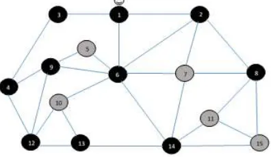
Let us illustrate an example of construction the CDS based on MIS. As we are looking for the optimal selecting of CDS, we outbalance for the agent to implement the second scenario to guarantee the optimal selecting of dominator node in the first iteration, even though this scenario induces additional movements by the agent Figure.1.
The agent starts the implementation of the algorithm in the node u=1, it randomly explores the
one-hop nodes vN1(u) that are adjacent to u. In
each node v, the agent explores all one-hop nodes
xN1(v) to calculate the degree of each node v. So,
in the first iteration the agent explores the one-hop nodes N1(1)={2,3,6} and visits the two-hop nodes N2(u)={4,5,7,8,9,10,14} of the node u, it marks them non-active white. Thus, the agent knows the degree of the node 1 and the degree of each one-hop neighbor nodes of 1, it select and adds the node 6 that has the largest degree D(6)=7 to the independent set,
IS={6}. The agent constructs the CDS
simultaneously with the selecting of independent nodes. Thus, it moves to the node 6, marks this node as dominator (Black) and the connected dominating set is CDS={6}. The agent moves to each one-hop neighbor nodes N1(6)={1,2,5,7,9,10,14} adjacent to node 6 in order to marks them as dominate (Gray), and explores each dominate (Gray) node. It moves to the one-hop neighbor nodes adjacent to each dominate (Gray) node to mark them as non-active white and calculate the degree of each dominate (gray) node. Since the agent explored the node 3 and it knew its degree, the agent changes the status of node 3 to active white. This active node becomes qualified to belong the independent set. Therefore, the resultant independent set is IS={6,3}. The agent moves to and marks the node 3 as dominator (Black) and all its adjacent non-active nodes as dominate
(gray), node 4, NNA(3)={4}, see Figure.1b. To
construct and guarantee the connection of the dominating nodes, the agent adds the dominate node 1 which is the parent node of the node 3 to the dominating set CDS={6,3,1} and changes the node 1 to dominator (Black). The agent then moves to each one-hop nodes adjacent to these selected
dominator nodes and marks them gray, see Figure.1c.
To start the next iteration, the agent selects and moves to the dominate (gray) node 14 that has the largest degree, D(14)=5, and the largest number of
non-active nodes DNA(14)=3, 3 non-active
nodes{11,13,15}, Figure.1d. This dominate node 14 does not allowed to be independent; it has one adjacent independent node 6. The agent moves to and explores each one-hop neighbor nodes N1(14)={7,11,13,15} adjacent to node 14 in order to select the optimal independent node. The resultant of this iteration is adding new independent node to the set IS, the node 13 which has one non-active nodes
DNA(13)=1, non-active nodes{12}, the independent
set becomes IS={6,3,13}, see Figure.1e. The agent marks the node 13 as dominator (Black), adds it to the connected the dominating set CDS={6,3,1,13} and changes its adjacent non-active node {12} to dominate (gray). To guarantee the connection of the dominating nodes, the agent adds the dominate node 14 which is the parent node of the node 13, that has the largest degree, to the connected dominating set CDS={6,3,1,13,14}, changes the nodes 14 to dominator (Black) and changes its one-hop active nodes {11,15} as dominate (gray), see Figure.1f.
The third iteration starts when the agent moves to the last active node 8. This node is explored, active and all its adjacent nodes are dominate (gray). Therefore, no one of these dominate nodes would be selected as independent node. The agent selects and adds the node 8 to the independent set IS={6,3,13,8}. It marks the node 8 as dominator (Black), adds it to the connected the dominating set CDS={6,3,1,13,14,8}. To guarantee the connection of the dominating nodes, the agent adds the dominate node 2 or node 7 to the connected dominating set CDS={6,3,1,15,14,8,7} which has the largest degree among all one-hop nodes adjacent to node 8, it selects and marks the nodes 7 as dominator (Black), see Figure.1(g).
At this point, the agent explores all the nodes in the graph. All the nodes of the graph G either dominating (Black) or dominate (gray), thus the agent successfully constructs the connected dominating set based on the maximal independent set, but this set is not minimum CDS as it consists of 7 nodes.
3.3. MA-CDS based on multipoint relays
60 [28] and then compare it with the extended greedy algorithm which proposed by Wu in [25] in which the free neighbor notation is introduced. In the first phase the agent applies one of these greedy algorithms in each node u to select the multipoint relay set denoted by MPR(u), we denote the first
instance by MA-OriginalGreedy and the second
instance by MA-ExtendGreedy algorithms.
Depending on the selected MPRs sets, the agent selects the CDS using two rules in the second phase.
Greedy Algorithm:
For each node u:
1. Add v ∈ N1(u) to MPR(u), if there is a node in
N2(u)covered only by v.
2. Add v ∈ N1(u) to MPR(u), if v covers the largest
number of nodes in N2(u) that have not been covered.
A node u selected as a member in the CDS if it is compatible with the following rules:
Rule 1: It has the largest degree than all its neighbors and it has two unconnected neighbors.
61
Figure.1:Constracting the CDS based on MIS algorithm.
IS ={} : the selected independent set at each iteration.
62
Extend Greedy Algorithm:
Wu’s EMPR [25] introduces a novel notation of free neighbor node in the EMPR. This notation originally introduced by using the node ID, Node v is a free neighbor of u if u is not the smallest ID neighbor of v. Chen and Shen in [22] observe that the node degree is more related to the size of the CDS instead of the ID. Therefore, based on this observation we replaced the ID by the degree of the
node in our implementation through
MA-ExtendGreedy algorithm. The node v is free neighbor of u, if u is not the largest degree neighbor of v, there is at least one neighbor of v has larger degree than u.
For each node u:
1. Add all free neighbors of the node u to the
MPR(u) set.
2. Apply the original greedy algorithm to the
residual one-hop neighbors to cover all remaining two-hop nodes.
A node u selected as a member in the CDS if it is compatible with the following rules:
Rule 1: It has the largest degree than all its neighbors and it has two unconnected neighbors.
3.3.1. Rule 2: the node is a multipoint relay selected by its neighbor that has the largest degree.
MA-OriginalGreedyAlgorithm:
Constructing the connected dominating set simultaneously with selecting each MPR set induces unacceptable number of agent moves. The agent needs to explore all one-hop nodes and visit all two-hop node to select the MPR of the node u, then it needs to explore all one-hop nodes and visit all
two-hop nodes of the node vN1(u), which has the
maximum degree.
Our algorithm goes in two phases, the first phase is applying the MPR heuristic algorithm to select the MPR set for each node and the second phase is globally applying the mentioned two rules. The agent selects a CDS based on the existing MPR set for each node that has generated using the original MPR heuristic algorithm. The used technique is to compute local MPR set formed in each node and then distributed in each node of the whole network to generate global CDS. The mobile agent applies the first phase to all nodes in the network, to selecte the MPR sets by the MPR heuristic algorithm. Then
the selected nodes as MPR become qualified to participate in the second phase to determine whether or not belong to the dominating set.
The agent in the node u intends to select a small multipoint relay set MPR(u) from the one-hop
neighbor nodes v N1(u). The whiteboard of each
node u in the graph contains of the N1(u), the selected MPR(u) nodes, the normal degree D(v) for
each node vN1(u), the exclusive degree Dexc(v) for
each node vMPR(u) and the selector nodes which
select the node u as one of their MPR nodes. The number of two-hope nodes of u, that be exclusively covered by v where v is an one-hop neighbor of u is Dexc(v).
To be more accurate, when the mobile agent explores a node u that means the agent visited all one-hop neighbor nodes of u, N1(u). Nodes announced themselves means that they exchange their one-hop nodes. Two adjacent nodes v1 and v2 can exchange their degree, and exclusive degree
Dexc(v1) and Dexc(v2) when the agent explores each
one-hop neighbor nodes of them N1(v1) and N1(v2). The mobile agent announces this information on behalf of those nodes. At the beginning, the agent does not rely on the degree of the visited nodes, the Basic criterion to select the MPR(u) of u is the
existence of one node or nodes x N1(v) that are
covered only by the node v N1(u) to calculate the
Dexc(v) for each node v N1(u).
MA-OriginalGreedy:
The agent in each node u performs the following steps:
The agent starts the iteration at a node u;
Visit and explore each one-hop nodes vN1(u)
of u;
Visit each one-hop nodes xN1(v) of v;
Calculate the normal degree D(v) and the Dexc(v;
Announce the information of the one-hop
neighbor nodes N1(v) to each xN1(v);
Calculate the two-hop nodes of u and select the
MPR(u) set;
Announce the information of the one-hop
neighbor nodes N1(u), selected MPR(u) nodes and their corresponding two-hop neighbor nodes
N2(u) to each vN1(u);
63
Selects the node vMPR(u) for the next iteration
which has largest Dexc(v), has maximum shared
one-hop nodes with the node u, and has the largest difference between its normal degree D(v) and the number of its one-hop nodes announced themselves to v.
In first iteration, the agent moves two hops from the current node u. It moves to each one-hop neighbor
node v N1(u). In each visited node v the agent
initiates the values of the normal degree of v, the exclusive degree of v and the one-hop selector nodes in the whiteboard and then starts the exploration. It explores the node v by visiting each adjacent nodes
x N1(v) to compute the two-hop nodes of u which
are exclusively covered by each node v. Thus, the agent knows the degree of each one-hop node
vN1(u). Whenever the agent completes visiting the
set nodes N1(v), it again moves to those visited
nodes x N1(v) in order to announce the
information of the one-hop neighbor nodes of the node v. Those information saved in the whiteboard
of each node x. Therefore, each node xN1(v) has
the N1(v) information. The agent could not
announces the N1(u) information to each node v
N1(u), unless the agent finishes exploring the set nodes N1(u) . The agent comes back to u, specifies the MPR set of u from N1(u), and computes the
exclusive degree Dexc(v) for each node vMPR(u).
Finally, it moves to those explored nodes v N1(u)
in order to announce the information of the one-hop nodes N1(u) and the selected MPR(u). The agent registers this information in the whiteboard of each
node vN1(u). It will registers the node u as a
selector in each node vMPR(u) that has been
selected to be multipoint relay. In this way, each
node vN1(u) knows the one-hop nodes of the node
u, those nodes represent the two-hop nodes for each other through the node u.
For the next iteration, we add additional constrains to select the node in which the agent starts
this iteration. The agent selects the node vMPR(u)
that has largest exclusive degree Dexc(v), has
maximum shared one-hop nodes with the node u, and has the largest difference between its normal degree d(v) and the number of its one-hop nodes announced themselves to v. Thus, we assumed that by adding this constrain the agent simultaneously computes the MPR set for more than one node in each iteration.
Whenever the agent visits node let’s say v1 that has been visited or explored in previous iteration,
v1 N1(v) and v1N1(u), the agent collects shared
information to compute the MPR for both nodes v and v1, it memorizes the N1(v) in the whiteboard of v1 and the N1(v1) in the whiteboard of v.
Until now, the agent does not know the degree of the two-hop nodes of the node u. With the progress of the algorithm, the agent may enter a two-hop node
x N1(v) that has the information of all its one-hop
nodes N1(x). The agent already visited this node x in different iterations. Thus, the agent computes the MPR set of node x and performs additional movements, it will move to all one-hop nodes of node x to announce the set of one-hop neighbor nodes N1(x) and its selected MPR(x) set. Following these procedure, the agent successfully select the optimal MPR nodes for each node in the graph and selects the CDS.
Let us illustrate an example of construction the CDS based on MPR set by the mobile agent. The agent starts the implementation of the algorithm in the node u=1, see Figure.2, it randomly explores the
one-hop nodes vN1(u) that are adjacent to u. In
64 multipoint relay for node 1 as it exclusively covers {5,9,10,14}, while node 2 selected as multipoint relay for node 1 as it exclusively covers {8} and node 3 selected as multipoint relay for node 1 as it exclusively covers {4}.
The agent then move to the node 6 according two criteria, node 6 has the largest exclusive degree among the one-hop nodes and it has the largest difference between its normal degree and the number of its one-hop nodes that it has their N1 information. The agent at each selected MPR node registers the information of the exclusive covered nodes, the exclusive degree, the information of one-hop nodes and the selectors nodes. After three iterations, the agent has visited all the nodes and has an overall vision, thus it can reach any node in the graph.
Finally, the agent be able to select the nodes that are qualified to belong to the CDS. The agent will use the two rules in the first instance and the notation of free neighbor with the two rules in the second instance. Actually, the agent by implementing those algorithms could not successfully construct the minimum connected dominating set. As we mentioned, the induced connected dominating nodes by those algorithms are large.
Figure.2 and table 1 explain the first phase for the first instance. Table 1 illustrates the generated MPR(u) sets for each node u based on the original greedy algorithm, the one-hop neighbor nodes,
two-hop neighbor nodes and the selectors nodes vN1(u)
which select u as MPR(v). All the nodes are selected as MPR except the nodes 5, 10, and 11, see the selectors column in the Table.1.
In the second phase, Rule1 and Rule2 applied to select the nodes belonged to the CDS, thus ten connected dominating nodes {1, 2, 3, 4, 6, 8, 9, 12, 13, 14} which their selectors have the largest degree and marked with red color in the Selectors column.
Table1: Multipoint relays set for each node of the graph in Figure.1a that is selected by the mobile agent based on the original greedy algorithm.
No
u MPR(u) N1(u) N2(u) Selectors
1 6,2,3 2,3,6 4,5,7,8,9,10,14 2,6,3
2 6,1,8 1,6,7,8 3,5,9,10,14,15 1,6,8
3 4,1 1,4 2,5,6,9,12 4,1
4 12,3,9 3,5,9,12 1,6,10,13 5,9,12,3
5 6,4 4,6 1,2,3,7,9,10,12,14 Null
6 14,9,2,1 1,2,5,7,9,10,14 3,4,8,11,12,13,15 1,2,5,7,9,10,14
7 6,14 2,6,8,14 1,5,9,10,11,13,15 14
8 2,15 2,6,15 1,6,11,14 2,15
9 6,4,12 4,6,12 1,2,3,5,7,10,13,14 4,6,12
10 6,12 6,12,13 1,2,4,5,7,9,14 Null
11 14,15 14,15 6,7,8,13 Null
12 4,9,13 4,9,10,13 3,5,6,14 4,9,10,13
13 14,12 10,12,14 4,6,7,9,11,15 12,14
14 6,7,13 6,7,11,13,15 1,2,5,8,9,10,12 6,7,11,13,15
15 14,8 8,11,14 2,6,7,13 8,11
3.3.2. MA-Extended Greedy Algorithm:
The agent in each node u performs the following steps:
The agent starts the iteration at a node u;
Visit and explore each one-hop nodes vN1(u)
of u;
Announce the information of N[u] to each node
vN1(u);
Calculate the normal degree D(u) and the normal
degree for each node vN1(u).
For each one-hop node vN1(u) except the node
that has the maximum degree:
Add the node u to the free neighbor set of v.
Select the node vN1(u), v has the maximum
degree among all the nodes vN1(u) to start the
next iteration;
End the iteration.
The agent starts the implementation of the algorithm in the node u=1, it randomly explores the
one-hop nodes vN1(u) that are adjacent to u. In
each node v, the agent explores all one-hop nodes N1(v) to calculate the degree of each node v. So, in the first iteration the agent explores the one-hop nodes N1(1)={2,3,6} and visits the two-hop nodes N2(1)={4,5,7,8,9,10,14} of the node 1. It adds the node 1 as a free neighbor in the free neighbor set of the nodes {2,3} except the node 6 as this node has the maximum degree among the nodes of N1(1), node 1 not free node of node 6. Then, the agent selects and moves to the node 6 to start the next iteration and repeats the same steps. It explores each non-explored one-hop nodes N1(6)={ 5,7,9,10,14}
and visits the two-hop nodes
65 explore any node that has its degree such node 1 and node 2. It adds the node 6 as a free neighbor in the free neighbor set of the nodes {1,2,5,7,9,10} except the node 14 as this node has the maximum degree among the nodes of N1(6). In this iteration, the agent visits all the nodes of the graph but does not explore all of them. In the third iteration the agent selects the node 14 which has the maximum degree among the nodes of N1(6), node 6 not free of the node 14 and repeats the same steps. After 6 iterations, the agent successfully explores all the nodes of the graph and selects all the free nodes for each node in the graph.
Figure.2 and table 2 illustrates the implementation of
the Extended Greedy Algorithmin the first phase for
[image:15.612.94.297.480.702.2]the second instance. The generated one-hop free neighbors for each node u are adding to the MPR(u) sets based on the Extended greedy algorithm. We observed that the new notation of free neighbor insufficient to cover the two-hop nodes for some nodes, e.g. node 2 does not select node 8 as free neighbor, even though node 15 covered only by node 8. Likewise, the same action in node 4, which does not select nodes 3 and 12, but those one-hop nodes selected by applying the original greedy algorithm in step two. Thus, this new notation adds additional nodes to the MPR sets.
Table 2: Multipoint Relays Set For Each Node Of The Graph In Figure.1a That Selected By The Mobile Agent
Based On The Extended Greedy Algorithm.
Node number
one-hop free
neighbors MPR(u) Selectors
1 2,3,6 2, 3, 6
2 1,6,7 8 1 , 6, 7, 8
3 1,4 1, 4
4 5,9 3,12 3, 5, 9, 12
5 4,6 4
6 Null 14,9,2,1 1, 2, 5, 7, 9, 10, 14
7 2,6,14 2, 8, 14
8 2,7,15 2, 15
9 4,6,12 4, 6, 12
10 6,12,13 12, 13
11 14,15 15
12 9,10,13 4 4, 9, 10, 13
13 10,12,14 10, 12,14
14 7 6,13 6, 7, 11, 13, 15
15 8,11,14 8 ,11
In the second phase, Rule1 and Rule2 applied to select the nodes belonged to the CDS, thus the same ten elected dominating nodes {1, 2, 3, 4, 6, 8, 9, 12, 13, 14} which their selectors have the largest degree and marked with red color in the Selectors column. Thus, those algorithms induce large number of dominating nodes whether we use the free neighbor notation or not. As well as, comparing to the original greedy algorithm that requires 38 selection, the extended greedy algorithm requires 46 selection in the process of electing the MPR nodes.
Figure.2: Selected Dominating Nodes By The Mobile Agent Based On The MPR Original And The MPR
Extended Greedy Algorithms.
4. CONCLUSION
In This work, we analyzed and evaluated the implementation of CDS construction based on the traditional marking, the MIS, and Multipoint Relays algorithms with slight modifications on those implemented algorithms to become appropriately used by the mobile agent. We discussed and made a comparison on the moves and iterations which performed by the agent and the final number of the constructed connected dominating nodes when the agent complete the CDS constructing. We believed that using the mobile agent has great promise
alternative way instead of exchange messages
approach.
66 starting at the same node in the same graph. The first used algorithm based on the MIS and the second based on the MPR to select the dominating nodes. We noted an excess in the number of moves that have made by the agent at the earlier iterations in the exploration phase and the agent selects large number of dominating nodes. Selected dominating nodes based on the MIS illustrates good result in the number of selected dominating nodes, but the agent performs more movements. Constructing the CDS based on MPR using the mobile agent is complicated and produces inappropriate additional dominating nodes and the agent performs additional moves to ensure the independence of the selected independent set and finally to ensure the connecting of the selected dominating nodes.
For implementing these algorithms, the mobile agent intends directly to enter the node that has the largest degree in each iteration to select the dominating nodes. Thus, the agent performs large number of movements, it then tries to link other nodes (nodes have to be covered) adjacent to the selected dominating node by visiting and exploring those nodes. This behavior adds additional selected dominating nodes.
Therefore, we need an efficient approach by which the agent achieves several goals, decreases the total number of agent moves; selects the minimum connected dominating nodes; and explores the nodes with minimum degree to select an appropriate dominating node for each node. As well as the direction of the interconnection among the nodes during the selection of the dominating node must be from the covered nodes toward the selected dominating node, which means every node has its opportunity to select and connect to the optimal dominating node. We assume by following this approach, the mobile agent will potentially perform fewer movements and reduce the total cost for exploring the graph. This is the motivations for the next work, and possibility of implementing those algorithms using Multi-agents taken into account for exploring large graph.
REFERENCE
[1] Ephremides, A., Wieselthier, J. E., & Baker, D.
J. (1987). A design concept for reliable mobile radio networks with frequency hopping signaling. Proceedings of the IEEE, 75(1), 56-73.
[2] Kim, D., Gao, X., Zou, F., & Wu, W. (2011).
Construction of fault-tolerant virtual
backbones in wireless networks. In Y. Xiao, F. H. Li & H. Chen (Eds.), Handbook of Security and Networks (pp. 465-486). Singapore: World Scientific.
[3] Wang, W., Kim, D., An, M. K., Gao, W., Li,
X., Zhang, Z., & Wu, W. (2013). On construction of quality fault-tolerant virtual backbone in wireless networks. IEEE/ACM Transactions on Networking, 21(5), 1499-1510.
[4] Li, Y., Wu, Y., Ai, C., & Beyah, R. (2012). On
the construction of k-connected m-dominating sets in wireless networks. Journal of Combinatorial Optimization, 23(1), 118-139.
[5] Zhang, N., Shin, I., Zou, F., Wu, W., & Thai,
M. T. (2008). Trade-off scheme for fault tolerant connected dominating sets on size and diameter. Proceedings of the 1st ACM International Workshop on Foundations of Wireless Ad Hoc and Sensor Networking and Computing (FOWANC’08). Hong Kong SAR, China (pp. 1-8).
[6] Sheu, P., Tsai, H., Lee, Y., & Cheng, J. (2009).
On calculating stable connected dominating sets based on link stability for mobile ad hoc networks. Tamkang Journal of Science and Engineering, 12(4), 417-428.
[7] Blum, J., Ding, M., Thaeler, A., Cheng, X.:
Connected dominating set in sensor networks and MANETs. In: Handbook of Combinatorial Optimization, Supplement vol. B, pp. 329–369. Springer, New York (2005).
[8] P S Vinayagam. A Survey of Connected
Dominating Set Algorithms for Virtual
Backbone Construction in Ad Hoc
Networks. International Journal of Computer Applications 143(9):30-36, June 2016.
[9] Jiguo Yu, Nannan Wang, Guanghui Wang, and
Dongxiao Yu. 2013. Review: Connected dominating sets in wireless ad hoc and sensor networks - A comprehensive survey. Comput. Commun. 36, 2 (January 2013), 121-134. DOI=http://dx.doi.org/10.1016/j.comcom.201 2.10.005.
[10] S. Guha and S. Khuller, Approximation
algorithms for connected dominating sets, Algorithmica, 20(4), pp. 374-387, Apr. 1998.
[11] X. Cheng, M. Ding, D.H. Du, and X. Jia, On
67
[12] K. M. Alzoubi, P.-J.Wan, O. Frieder: Maximal
Independent Set, Weakly Connected
Dominating Set, and Induced Spanners for Mobile Ad Hoc Networks, International Journal of Foundations of Computer Science, Vol. 14, No. 2, pp. 287-303, 2003.
[13] S. Butenko, X. Cheng, D.-Z. Du, and P.M.
Pardalos, On the construction of virtual backbone for ad hoc wireless networks, In S. Butenko,R. Murphey, and P.M.Pardalos,
editors, Cooperative Control: Models,
Applications and Algorithms, pp. 43-54, Kluwer Academic Publishers,2003.
[14] Y. Li, M.T. Thai, F. Wang, C.W. Yi, P.J. Wan,
D.Z. Du, On greedy construction of connected dominating sets in wireless networks, Wireless Communications and Mobile Computing 5 (8) (2005) 927–932.
[15] X. Cheng, M. Ding, and D. Chen, An
approximation algorithm for connected dominating set in ad hoc networks, Proc. of International Workshop on Theoretical Aspects of Wireless Ad Hoc, Sensor, and Peer-to-Peer Networks (TAWN), 2004.
[16] K.M. Alzoubi, P.-J. Wan and O. Frieder,
Distributed Heuristics for Connected
Dominating Sets in Wireless Ad Hoc Networks, Journal of Communications and Networks, Vol. 4, No. 1, Mar. 2002.
[17] Cidon and O. Mokryn, Propagation and Leader
Election in Multihop Broadcast Environment, Proc. 12th Int. Symp. Distr. Computing, pp.104-119, Greece, Spt. 1998.
[18] F. Dai and J. Wu, An Extended Localized
Algorithm for Connected Dominating Set Formation in Ad Hoc Wireless Networks, to appear in IEEE Transactions on Parallel and Distributed Systems, 2004.
[19] S. Butenko, X. Cheng, C. Oliveira, and P.M.
Pardalos, A new heuristic for the minimum connected dominating set problem on ad hoc wireless networks, In S. Butenko, R. Murphey,
and P.M. Pardalos, editors, Recent
Developments in Cooperative Control and Optimization, pp. 61-73, Kluwer Academic Publishers, 2004.
[20] B. Mans and N. Shrestha, “Performance
Evaluation of Approximation Algorithms for Multipoint Relay Selection,” Med-Hoc-Net 2004, 3rd Annual Mediterranean Ad Hoc Net. Wksp., Bodrum, Turkey, June 27–30, 2004.
[21] N. Shrestha, “Performance Evaluation of
Multipoint Relays:Collision and Energy Efficiency Issues,” Macquarie University, Tech. Rep., 6 Apr. 2003.
[22] Xiao Chen and Jian Shen, "Reducing
connected dominating set size with multipoint relays in ad hoc wireless networks," 7th
International Symposium on Parallel
Architectures, Algorithms and Networks, 2004. Proceedings., 2004, pp. 539-543.
[23] C. Adjih, P. Jacquet, and L. Viennot,
“Computing connected dominated sets with multipoint relays”, Technical Report, INRIA, Oct. 2002.
[24] O. Liang, Y. A. Sekercioglu and N. Mani, "A
survey of multipoint relay based broadcast schemes in wireless ad hoc networks," in IEEE Communications Surveys & Tutorials, vol. 8, no. 4, pp. 30-46, Fourth Quarter 2006.
[25] J. Wu, “An enhanced approach to determine a
small forward node set based on multipoint relays”, accepted to appear in Proc. of 2003 IEEE Semiannual Vehicular Technology Conference (VTC2003- fall), Oct. 2003.
[26] V. Chvatal, A Greedy Heuristic for the
Set-Covering Problem, Mathematics of Operation Research, 1979, ch. 4, pp. 233–35.
[27] Kim, D., Wu, Y., Li, Y., Zou, F., & Du, D. (2009). Constructing minimum connected dominating sets with bounded diameters in wireless networks. IEEE Transactions on Parallel and Distributed Systems, 20(2), 147-157.
[28] A. Qayyum, L. Viennot, and A. Laouiti,
“Multipoint relaying for flooding broadcast message in mobile wireless networks”, Proc. HICSS-35, Jan. 2002.
[29] W. Abdou, N. O. Abdallah and M. Mosbah,
"ViSiDiA: A Java Framework for Designing, Simulating, and Visualizing Distributed Algorithms," Distributed Simulation and Real Time Applications (DS-RT), 2014 IEEE/ACM 18th International Symposium on, Toulouse, 2014, pp. 43-46.
[30] Philip Levis , David Culler, Maté: a tiny virtual
machine for sensor networks, Proceedings of the 10th international conference on Architectural support for programming languages and operating systems, October
05-09, 2002, San Jose,