Multiplicatively separable preferences and output persistence

Vaona,

A. (2005) Multiplicatively separable preferences and output

persistence. Working Paper. Birkbeck, University of London, London, UK.

Downloaded from:

Usage Guidelines:

Please refer to usage guidelines at

or alternatively

Birkbeck Workin

g

Pa

p

ers in Economics & Finance

School of Economics, Mathematics and Statistics

BWPEF 0511

Multiplicatively Separable

Preferences and Output Persistence

Andrea Vaona

December 2005

Abstract

In the New-Neoclassical Synthesis literature it is customary to use additively separa-ble preferences, very often not compatisepara-ble with long-run productivity growth and trend in‡ation. The present paper shows that using multiplicatively separable preferences it is possible to gain further insight on the persistence mechanics of this class of models. In particular it is showed that the more leisure and the money-consumption bundle are Edgeworth complement and the less persistent are output deviations after a monetary shock. The basic intuition for this result is that an increase in money supply not only induces economic agents to increase their labour supply, but also raises the opportu-nity cost for this choice given that agents with more money in their pockets and greater consumption would like to have more leisure too. In addition, empirical estimates not only support multiplicatively and not additively separable preferences, but highlight new problems for the New-Neoclassical Synthesis given that leisure and money (consumption) appear to be Edgeworth complements and not substitutes.

K eyw ords: O utput p ersistence, multiplicatively separable preferences.

JE L classi…cation : E31, E40

1. Introduction

The persistence puzzle has been at the centre of a large debate among econo-mists. Chari, Kehoe and McGrattan (2000) (hereafter CKM (2000)) and Ascari (2000) argue that, for reasonable values of the structural parameters, Dynamic General Equilibrium Models with either price staggering or wage staggering have considerable di¢ culties in displaying output persistence after an increase in money supply. On the other hand Erceg (1997), Andersen (1998) and Huang and Liu (2002) have argued that there is a crucial di¤erence between price staggering and wage staggering models, whereby the latter ones have a greater ability in mimicking the stylised fact of output persistence than the former ones. However, Rotemberg and Woodford (1997) produced output persistence with price staggering. Finally Edge (2002) and Ascari (2003) argued that the ability of a model to produce out-put persistence is not due to either price or wage staggering but to other features of the model, such as …rm speci…c factors and the immobility of labour, which are the basic characteristics of the most successful models produced by the persistence literature so far: the "yeoman farmer" model and the "craft unions" model.

In particular, the "yeoman farmer" model assumes the existence of a set of mo-nopolistically competitive producers with speci…c labour inputs, while the"craft unions" model assumes the existence of a set of monopolistically competitive unions that set the wage for the households belonging to di¤erent crafts. The basic intuition for their better persistence performance is that agents do not want to miss the demand for their speci…c kind of product or labour to the bene…t of their competitors locked in past contracts and therefore they choose not to raise the price for their good or labour too fast. To the purpose of my analysis, I will therefore focus on the "craft unions" model and the "yeoman-farmer model".

Moreover Ascari (2004) has recently shown that the short run properties of the Calvo model are not robust to trend in‡ation whereas those of the Taylor model are, so I will stick to Taylor staggering. In this contribution I will adopt the widespread method of log-linearising the system of the …rst order conditions around a zero in‡ation steady state, cutting the money intertemporal link but assuming wage/price stickiness and exploring the persistence properties of a stripped down version of the model that can be solved analytically. I will then present numerical evidence for the full scale model, once reinserting the money intertemporal link.

To my knowledge the signi…cance of the assumption of additively separable preferences for the performance of the new Keynesian models with staggered prices/wages has not been thoroughly investigated, notwithstanding that both Woodford (2003) and Walsh (2003) called for a sound assessment of this issue.

the economic system. Indeed, each of the utility arguments - money, consumption and leisure - will enter not only its own marginal utility but also the marginal utilities of the other two. This property is of course appealing to those thinking to social and economic phenomena as deeply interlinked. Moreover, it will allow to assess thoroughly how preferences and technology interact in the persistence mechanics of neo-keynesian models, an issue where the assumption of additively separable preferences induces too simplistic results.

It is worth also noting that the separability of utility function and detrending are deeply connected: as it is possible to show following King and Rebelo (2000) an additively separable utility function is not always compatible with a steady state with either a positive in‡ation rate or productivity growth, unless speci…ed as a logarithmic Cobb-Douglas. I will compare multiplicatively separable preferences to additively separable ones also regarding the e¤ect of steady state money growth on output persistence.

Finally multiplicatively separable preferences are important not only for their theoretical implications but also on the empirical ground. There are not many empirical studies estimating preferences including leisure, due to the di¢ culty in …nding data about working-time especially at the aggregate level and for sizeable samples. However, to my knowledge there exists one study trying to accomplish this task.

Soriano de Alencar and Nakane (2003) estimated the Euler equations deriving from a multiplicatively separable utility function, showing its greater ability to match their data with respect to additively separable preferences and …nding a positive value for the elasticity of the marginal utility of leisure with respect to money and consumption, implying their Edgeworth complementarity.

This is bad news for the ability of neo-keynesian models to display persistence of output deviations from steady state after a monetary shock. Indeed, by using a utility function similar to that in King, Plosser and Rebelo (2001), I will show that in the craft unions and in the yeoman-farmer model the persistence of output after a monetary shock decreases the more leisure on the one hand and money and consumption on the other are Edgeworth complements. The underlying reason is that, as showed in Ascari (2003), due to labour immobility, in those models eco-nomic agents will not change their price/wage after a monetary shock to preserve their demand and will increase their labour supply, but the increase in money bal-ances and consumption will increase the marginal utility of leisure increasing the opportunity cost of persistent deviations of output from steady state. What is also interesting is that the restrictions imposed by a utility function à la King, Plosser and Rebelo (2001) result in making the labour market the centre of persistence issues, excluding that other parts of the economic system may have a role.

the full scale version of the model, the half life of the output deviation from steady state, de…ned as the time it takes to shrink to half of its impact value. Ascari (2003) focused on the root of the system. Dealing with unemployment issues, Karanassou, Sala and Snower (2003) used the sum of the area below the impulse response function of unemployment to measure how persistent are unemployment changes after shocks in competitiveness, social security bene…ts and the real interest rate. In this contribution I will focus on the root of the system for the stripped down version of the model and the area below the impulse response function of the output deviation from steady state for the full scale model, because I think that the right question in the present context is not what is the intensity of the output deviation in each period compared to its impact value but how much product is possible to gain after a monetary shock.

To sum up the proposed study will attempt to take further the analysis of the persistence mechanics of new-keynesian models with sticky wages and prices by exploring how multiplicatively separable preferences a¤ect output persistence in the "craft unions" model and in the "yeoman farmer" model without intertemporal links but the staggered wage/price by means of both symbolic and numerical analysis. In this contribution I adopt a Money in the Utility function approach and not a Cash-In-Advance one, however they have been showed to be functional equivalent (Walsh, 2003).

The rest of the paper is structured as follows. Section 2 shows closed form solutions for stripped down versions of both the "yeoman farmer" model and the "craft unions" model. All the technical steps to achieve these solutions are in the Appendices to the paper. Section 3 shows how the root of the system changes as a function of the underlying structural parameters. Section 4 shows numerical results for the full scale "craft unions" model. Section 5 concludes.

2. The Stripped-Down Version of the Models

2.1. The Craft Unions Model

I suppose the existence of four markets: the intermediate and the …nal labour markets and the intermediate and the …nal product markets. In the intermediate labour market, a continuum of monopolistically competitive households, indexed by i ₂ [0;1], sell their speci…c labour force (Hit) to perfectly competitive

inter-mediaries at the wage rate Wit. Through the …nal labour market, the labour

intermediaries provide a continuum of monopolistically competitive …rms, indexed by j ₂ [0;1], on the intermediate product sector with an homogeneous labour supply (Ht) charging them the price of the wage index (Wt). Firms buy the

ho-mogenous labour input and sell a di¤erentiated output (Yjt) for the pricePjt to

Therefore there will be two markets with monopolistic competition, the interme-diate labour and product markets, and two markets with perfect competition, the …nal good and labour markets.

To each market corresponds one maximization problem. Labour intermediaries maximize their production subject to the constraint that their output market is perfectly competitive:

max

Hit

Ht=

Z 1 0 H w 1 w it di w w 1

s:t: WtHt

Z 1

0

WitHitdi= 0

where w is the elasticity of substitution between di¤erent kinds of labour.

Solving the maximization problem above it is possible to obtain the demand for the individual kinds of labour

Hit=

Wit

Wt

w

Ht (1)

and the aggregate wage index:

Wt=

Z 1

0

W1 w

it di

1

1 w

(2)

Assuming wage staggering and the existence of two labour cohorts, (2) can be rewritten as

Wt=

1 2W 1 w it + 1 2W 1 w it 1 1 1 w

given that due to symmetry all the households within a cohort set the same wage. The …nal sector problem mirrors the problem above given that the …nal sector producers maximize their production having a perfectly competitive output market and monopolistically competitive input market

max

Yjt

Yt=

Z 1 0 Y p 1 p jt dj p p 1

s:t PtYt

Z 1

0

PjtYjt dj= 0

By solving this maximization problem it is possible to obtain the usual demand function for individual output

Yjt=

Pjt

Pt

p

Yt (3)

and the aggregate price index

Pt=

Z 1

0

P1 p

jt dj

1

1 p

(4)

In the intermediate product market, each …rm maximizes its pro…t under the constraints of the production function and the demand function for their output:

max

Pjt

PjtYjt WtHjt

s:t Yjt= Hjt (5)

Yjt=

Pjt

Pt

p

Yt

where Hjt is the demand for labour of …rmj. The solution to (5) gives the price

setting equation:

Pjt=

1 1 _p

p 1

WtY

1 ₁

jt (6)

where due to the absence of price staggering Pjt = Pt and Yjt = Yt: This also

impliesHjt=Ht

Finally the representative consumer maximizes her utility given the budget constraint, the individual labour demand and the resource constraint:

max fCt; Mt_Pt;Witg

1

X

t=0

t_{U C} t;

Mt

Pt

;1 Hit

s:t: PtYt=PtCt+Mt tMt 1+Bt Bt 1

PtYt=

Z 1

0

WitHitdi+Pt t (7)

Hit=

Wit

Wt

w

Ht

Mt+Bt=PtYt PtCt+ tMt 1+Bt 1

and the government budget constraint is

PtGt=Mt+Bt tMt 1 Bt 1

I further suppose that money is growing in steady state at the rate and that nominal wages grow at the same rate too. So in fact, agents when maximizing utility choose a growth path for their wage.

After detrending nominal variables, (7) becomes

max fCt; Mt_Pt;Witg

1

X

t=0

t_{U C} t;

mt

pt

;1 Hit

s:t: ptYt=ptCt+mt t

mt 1

+bt

bt 1

ptYt=

Z 1

0

witHitdi+pt t (8)

Hit=

wit

wt

w

Ht

where small case letters are the detrended counterpart of the capital ones. The existence of wage staggering appears clear considering the wage …rst order condi-tion, which is obtained by maximizing utility subject to the constrains showed in (7) with respect to the household wage hold …xed over the contract period:

Et

"

UH(t) w

wit

wt

w

Ht

wit

+ UH(t+1) w

wit

wt+1

w

Ht+1

wit+1 #

=

=Et

"

t( w 1)

wit

wt

w

Ht

pt

+ t+1 ( w 1)

wit

wt+1

w

Ht+1

pt+1 #

CCc^t+ CM( ^mt p^t) + CH^hit ^t= 0 (9)

E M C^ct+ M M( ^mt p^t) + M H^hit ^t+ ^t+1 = 0 (10)

E[ _HC(^ct+ ^ct+1) + HM( ^mt p^t+ m^t+1 p^t+1) +

+ _HH ^hit+ ^hit+1 (1 + ) ^wit ^t ^t+1+ ^pt+ p^t+1 i

= 0 (11)

^

hit w( ^wt w^it) h^t= 0 (12)

^

yt

C Yc^t

m

Y m^t (1

1 )^pt

^

mt 1

= 0 (13)

^

wt

1

2( ^wit+ ^wit 1) = 0 (14) ^

pt w^t

1 ^

yt= 0 (15)

^

yt ^ht= 0 (16)

where the variables without time subscript are steady state variables.

To achieve the stripped down version of the model above it is necessary to cut the money intertemporal link, which is the same as to set =₁: a simpli…ca-tion that will be eliminated when going back to the full scale model. After this operation the money …rst order condition (10) becomes:

M Cc^t+ M M( ^mt p^t) + M H^hit= ^t

and the budget constraint

^

yt=

C Y^ct+

m

Y ( ^mt p^t) By the same token in steady state one will have:

Y =c+m

p

In this way, the system can be solved even without an equality between real money holdings, consumption and income as in CKM (2000). Furthermore, it seems inappropriate also to solve separately the Euler equation of money as a Bellman equation as in Ascari (2003) given that it results in unnecessarily re-stricting the product between the quantity of real money and the utility deriving from consumption . As showed in the Appendix, after a few passages and keeping in mind that ^hjt+1 = w( ^wjt w^t+1) + ^ht+1 it is possible to obtain a system

^

wjt =

1

2(^pt+Etp^t+1) + 1

2 (^yt+Ety^t+1) ^

pt =

1

2( ^wjt+ ^wjt 1) +ay^t (17) ^

yt = 1m^t+ 2p^t+ 3w^jt

with the parameters assuming the following forms: 1 = b1 1+b0 b0

w(1 )

; 2 =

b1+b0 w

1+b0 b0

w(1 )

; 3= b0 w 1+b0 b0

w(1 )

; =

h_a

0

b₁+1 a1 a0b₁b0 +

1 i

h

a1 a0bb01 w+1

i 1 ; a=

1 _{; where we have b}

1 = C_Y M M CM

CC M C +

m

Y; b0 = C Y

M H CH

CC M C ;

a0= h

( _{HC M C})( M M CM)

( CC M C) + ( HM M M) i

; a1= h

( _{HC M C})( M L CL)

( CC M C)+ ( HH M H) i

where _IJ = UIJ( )

UI( )J.

It is interesting to note that the last equation of the system above can be written also in the following form:

^

yt=

b1

1 +b0( ^mt p^t) +

b0

1 + b0 w( ^wt w^jt) (18)

therefore the distance of output from its steady state value is a function of the distance of real money from its steady state level plus a factor depending on the ine¢ ciencies arising from staggered wage(price)-setting during transitional dynam-ics.

It is possible to consider the following utility function which is consistent with steady state real and nominal growth:

U = 8 > > < > > : 1 1 c h

cCt + (1 c) MPtt

i1 1 c

v(Lit) if c6= 1

lnh cCt + (1 c) MPtt i1

+v(Lit) if c= 1

(19)

where Lit = 1 Hit and v(Lit) = ₁₊1 1 L1+it , decreasing and convex for

c >1; andv(L) = 1+1 L 1+

it 1 , increasing and concave otherwise - in order

to make sure that leisure, money and consumption are goods, as in King, Plosser and Rebelo (2001).

The utility function above imposes three restrictions on the parameters of (17):

M M CM= CC M C (20)

M H = CH (22)

It is worth stressing that the restrictions above allow an easy solution for (17), given that imposing them it is possible to obtainb0= 0; b1 = C_Y +m_Y = 1due to

the budget constraint,a0= 1, a1 = LL CH. So that the system to be solved

is:

^

wjt =

1

2(^pt+Etp^t+1) + 1

2 (^yt+Ety^t+1) ^

pt =

1

2( ^wjt+ ^wjt 1) +ay^t (23) ^

yt = m^t p^t

with = 1+

a_{1 +1}

1+ wa1

1 _anda=1

Adopting standard methods (Sargent, 1987 and Ascari, 2003) and exploiting the restrictions (20)-(22), it is possible to show that the persistence root of the system is a decreasing function of the following term:

RCU =

a+

a+ 1 =

( _{HH M H}) + 1 ( _{HH M H}) w+ 1

=

1 + H

1 H+

(1+ )L

(L1+ ₁₎H 1 + ₁H_H +₍(1+ )_L1+ L₁₎H w

(24)

where H is the steady state value of labour supply. It is worth recalling that the root of the system is 1 pR

1+pR: The dependence of persistence on the steady state

value ofH is common to the additively separable utility function given that M H

and CH are equal to zero in that case. I will return to the derivative of the R-term

above after brie‡y considering the yeoman-farmer model.

2.2. The Yeoman-Farmer Model

max

fCt; Mt_Pt; Pjt; Btg

1

X

t=0

t_{U C} t;

Mt

Pt

;1 Hjt

s:t:Hjt=

1

Y

1

jt

PtYt=PtCt+Mt tMt 1+Bt Bt 1

Yjt=

Pjt

Pt

w

Yt

After detrending, taking …rst order conditions for both the maximization problem above and for that of the …rms of the …nal product sector, log-linearising the system of equations obtained in this way and after a few passages (see the Appendix), it is possible to arrive to an Ascari-like system as above withpjt instead ofwjt and

with the following parameters: 1 = b1

1+b0; 2 =

b1+b0 p

1+b0 ; 3 =

b0 p

1+b0; =

a0

b1+1+

b0_+a 1 1+ p ab01b0 a1

; a = 0; b1 = C_Y M M CM

CC M C +

m Y; b0 =

C Y

M H CH

CC M C ; a0 =

( _{LC M C}) M M CM

CC M C +( LM M M); a1= ( LC M C)

M L CL

CC M C

1

+ 1 ₍

LL M L 1 + ):

As in the previous case it is possible to show that the R of the system is:

RY F =

a+

a+ 1 =

1 + 1

HH 1 CH+1 1

1 + 1

HH 1 CH+1 1 p

=

1 + 1 H

1 H +

1 (1+ )Lit

(L1+it 1)

H+1 ₁

1 + 1 H

1 H+

1 (1+ )Lit

(L1+it 1)

H+ 1 ₁

p

3. Persistence as a function of preferences and technology

It is worth studying the sign of the derivatives of the R-terms above in order to understand how the values of the structural parameters a¤ect persistence, recalling that the persistence root of the system is a decreasing function of the R-term and therefore what increases R will decrease persistence and viceversa.

From the equations above it is straightforward to see that

@Ri

@ _HH <0if j>1withi=CU; Y F andj=w; p (25) where _HH is the inverse of the intertemporal elasticity of substitution of leisure times the ratio between working time and leisure (see the Appendix). Therefore like in Ascari (2003) the intuition that a high intertemporal elasticity of substitu-tion of leisure is necessary to obtain persistence may or may not hold. However, it does hold to the condition that the intratemporal elasticity of substitution be-tween di¤erent kinds of labour/goods is big enough. The intuition is that economic agents in presence of monopolistic competition and a high substitutability of dif-ferent kinds of labour/goods do not want to miss the temporary increase in output after a monetary shock to the bene…t of their competitors and therefore they do not raise their price quickly. In addition given the high intertemporal substitutability of leisure they will try to reap the largest possible bene…t from the temporary increase in demand.

As far as the degree of complementarity between money (consumption) and leisure the following result holds:

@Ri

@ _CH >0 if j>1withi=CU; Y F andj=w; p (26)

Therefore, the more leisure and money (consumption) are Edgeworth complements and the more persistence will decrease because in this context where money and consumption can a¤ect the marginal utility of leisure, an increase in the quantity of money will increase the marginal utility of leisure and it will reduce persistence, by reducing labour supply.

Regarding w, p and ,

@RCU

@ w

>0if _{M H} 1< _HH < _{M H} (27)

@RY F

@ p

>0if _{M H} 1< _HH < _{M H} 1 + (28)

@RY F

@ <0if M H 1> HH (29)

An increase of p, w, increases persistence unless HH lays in an interval

The economic meaning of the results regarding p, w and is well known

in the literature. Ascari (2003) already showed that large values of the elasticity of substitution between di¤erent goods or kinds of labour increase persistence, because, as already stated, economic agents do not raise price quickly to avoid that competitors with prices/wages set in previous periods steal them demand. On the other hand, an increase in the elasticity of the production function with respect to labour inputs increases persistence because small changes in labour supply can produce large changes in output. The results above show that this is not the whole story and that economic agents face a trade-o¤ in their preferences as long as money (consumption) and leisure are complement because on the one hand they will try not to miss the demand for their speci…c kind of good (labour) but on the other they will be tempted to take advantage from the increase in their money holdings by reducing their labour supply. In the same way a large increase in output, in presence of a very elastic production function, will increase money holdings (given that in this model money supply and money demand are always equal), reducing labour supply and therefore persistence.

Finally, also the issue if price staggering or wage staggering generates more per-sistence depends on the value of the underlying parameters, under the hypothesis that p= w:

RCU > RY F if p= w>1; <1 and LL > M L 1 (30)

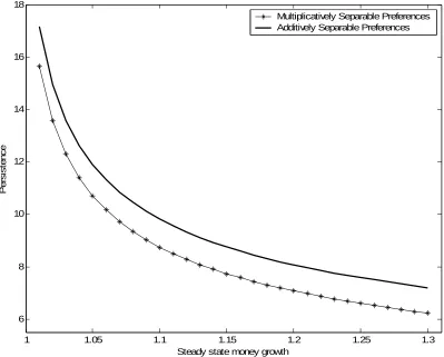
In order to appreciate the magnitude of the e¤ect of multiplicatively separable preferences on output persistence, Figure 1 shows the root of the system of the "craft unions" model as a function of w: As expected output persistence is

in-creasing in w, but persistence overestimation deriving from additively separable

preferences, though been sizeable, does not substantially depend on the elasticity of substitution between di¤erent kinds of labour.

4. The full scale version of the model

This section tackles the issue of the incidence of additively versus multiplica-tively separable preferences on the persistence of output deviations from steady state after a monetary shock in the context of the full scale "craft unions" model. When moving to consider the full scale version of the model from the stripped down one, it is necessary to reinsert the money intertemporal link. I will now also suppose that the money shock takes place at the end of periodtso that households’ asset move according to the following law of motion:

Therefore the log-linearized system of equations will be very similar to (9)-(16), with a few exceptions. The …rst order condition with respect to money will be replaced by:

Et M C^ct+ M M(^t+ ^mt p^t) + M H^hit ^t+ ^t+1 = 0

the budget constraint by

^

yt

C Y^ct

m

Y m^t+ ^t (1

1 )^pt

^

mt 1

= 0

The …rst order condition with respect to consumption will be replaced by:

CCc^t+ CM(^t+ ^mt p^t) + CH^hit ^t= 0

and the …rst order condition with respect to the household wage by:

E[ _HC(^ct+ ^ct+1) + HM( ^mt+ ^t p^t+ m^t+1 p^t+1) +

+ _HH ^hit+ ^hit+1 (1 + ) ^wit ^t ^t+1+ ^pt+ p^t+1 i

= 0 (31)

^_tis supposed to follow an AR(1) process.

^_t= ^_{t 1}+ ^t

To …nd the steady state, let us assume like in King, Plosser and Rebelo (2001), thatH = 0:3. As a consequence, one has thatHi =H andLi= 1 H:Considering

the aggregate production function of the intermediate output sector it is possible to obtain the level of output

Y = H

and, therefore, by using the money and the consumption …rst order conditions, the level of consumption and that of money holdings

Y =C+ (1 1) (1 ) c (1 c)

1 1

C

m= (1 ) c (1 c)

1 1

C

Finally, by combining the wage and consumption …rst order condition it is pos-sible to obtain the parameters of a generalized version ofv(Lit)to be set

v(L) =

1 + L

1+ ₁

because is not identi…ed, given that combining the wage and the consumption …rst order conditions it cancels out. Therefore, I switched to the following function of leisure

v(L) = 1 1 + L

1+

where is set endogenously:

=L1+ 1 +

1 c

(L) w ( w 1)

1 1 _p

p 1

Y 1 1

8 < :

cC 1

h

cC + (1 c) MP

i 9 = ;

1

Of course the number of parameters does not change with respect to King and Rebelo (2000).

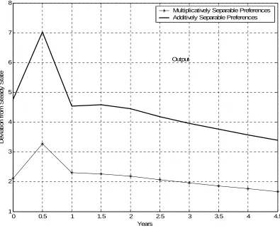
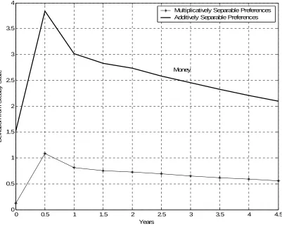
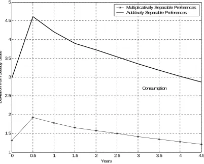
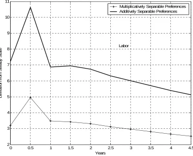
The model was calibrated using standard parameter values showed in Table 1. The results about output persistence after a monetary shock are showed in Figure 2. Measuring output persistence as the area below the impulse response function of output, it is clear that additively separable preferences entail a substantial over-estimation of persistence, due to the fact that economic agents are more willing to supply labour (Figure 3) and, therefore, they can have more money and consump-tion (Figures 4 and 5). Once the trade o¤ between money and consumpconsump-tion, on the one hand, and leisure, on the other, can play a role thanks to the introduction of multiplicatively separable preferences, the deviation from steady state of labour is far less marked, together with those of consumption and money.

Table 2 shows the result of a sensitivity analysis regarding the overestimation of the persistence of output deviation from steady state due to the adoption of additively separable preferences for di¤erent values of , w; and . Persistence

overestimation was measured in this exercise as the di¤erence between the sum of the area below the output impulse response function of a model with additively separable preferences and that with multiplicatively separable preferences. The results point again to a substantial overestimation that grows dramatically with the intertemporal elasticity of substitution of leisure and less markedly with the elasticity of substitution between di¤erent kinds of labour. Also an increase in increases overestimation, while the contrary happens for an increase in steady state money growth, though in these two cases the involved changes are not sizeable.

the root of the system. The underlying intuition for this result is that the higher is steady state money growth and the less incentive have economic agents to let past contracts survive. Technically, this is conveyed by the fact that detrending reduces the weight of past variables with respect to current and future ones, reducing their ability to a¤ect the system dynamics.

5. Conclusions

In the present contribution, I addressed the issue of what are the consequences of taking into consideration multiplicatively and not additively separable prefer-ences for output persistence after a monetary shock in a neo-keynesian framework. The most general result is that persistence will decrease the more leisure on one hand and money and consumption on the other are Edgeworth complements, be-cause economic agents will face a trade-o¤ that is impossible to grasp by using additively separable preferences. Namely, in presence of labour immobility, after a monetary shock on the one hand they will raise the price for their product/wage slowly not to miss the increase in demand to the bene…t of their competitors, on the other the increase in their money holdings will raise the marginal utility of leisure and reduce their labour supply.

References

Andersen, T. M. (1998), "Persistency in Sticky Price Models",European Economic Review. Papers and Proceedings 42, 593–603.

Ascari, G. (2000), "Optimising Agents, Staggered Wages and the Persistence of the Real E¤ects of Money",The Economic Journal 110, 664-686.

Ascari, G. (2003), "Price/Wage Staggering and Persistence: A Unifying Frame-work",Journal of Economic Surveys, 17-4. pp. 511-40.

Ascari, G. (2004), "Staggered Prices and Trend In‡ation: Some Nuisances", Re-view of Economic Dynamics, 7-3, pp. 642-67.

Chari, V., P. Kehoe and E. McGratten (2000), "Sticky Price Models of the Busi-ness Cycle: Can the Contract Multiplier Solve the Persistence Problem?", Econometrica68, 1151-1179.

Edge, R. M. (2002), "The Equivalence of Wage and Price Staggering in Monetary Business Cycle Models",Review of Economics Dynamics5, 559-585.

Erceg, C. (1997), "Nominal Wage Rigidities and the Propagation of Monetary Disturbances", Board of Governors of the Federal Reserve System.

Huang, K. X. D. and Z. Liu (2002), "Staggered Price-Setting, Staggered Wage-Setting and Business Cycle Persistence", Journal of Monetary Economics 49 (2002), 405–433.

Karanassou, M., H. Sala and D. Snower (2000), "Unemployment in the European Union: Institutions, Prices and Growth", IZA DP 899.

King, R. G. and S. T. Rebelo, (2000) "Resuscitating Real Business Cycles", Rochester Center for Economic Research, Working Paper No. 467.

King, R. G., C. I. Plosser and S. T. Rebelo, (2001), "Production, Growth and Business Cycles: Technical Appendix", mimeo.

Rotemberg, J. J. and M. Woodford (1997), "An Optimization Based Econometric Framework for the Evaluation of Monetary Policy", in J. J. Rotemberg and B. S. Bernanke (Eds.), NBER Macroeconomics Annual 1997, pp. 297–346, Cambridge, MA, The MIT Press.

Sargent, T. (1987),Macroeconomic Theory, Boston MA, Academic Press.

Walsh, C. E. (2003),Monetary Theory and Policy, The MIT Press, London.

A Appendix

A1. The Utility Function

In order to shed more light on the restrictions (20) to (22), the …rst part of this Appendix is devoted to the properties of the utility function. Let us suppose that c<1;so that the utility function is

U = 1

1 c

(

cCt + (1 c)

Mt

Pt

1)1 c

1 1 + L

1+

it 1 (32)

whereLis leisure andLit= 1 Hit:

So by taking …rst derivatives, it is possible to obtain:

UC =

(

cCt + (1 c)

Mt

Pt

1)1 c

cCt 1

1 1 + L

1+

it 1

UM =

(

cCt + (1 c)

Mt

Pt

1)1 c

(1 _c) Mt

Pt

1

1 1 + L

1+

it 1

UL =

1

1 c

(

cCt + (1 c)

Mt

Pt

1)1 c

(Lit)

Note also thatUL = UH, whereUH is the marginal disutility of labour. By

taking second order derivatives and recalling that _IJ = UIJ( )

UI( )J; it is possible to

CC = (1 c ) cCt + (1 c)

Mt

Pt

1

cCt + 1

CM = (1 c ) cCt + (1 c)

Mt

Pt

1

(1 c)

Mt

Pt

CH =

(1 + )L_it L1+_it 1

H

M M = (1 c ) cCt + (1 c)

Mt

Pt

1

(1 _c) Mt

Pt

+ 1

M C = (1 c ) cCt + (1 c)

Mt

Pt

1

cCt

M H =

(1 + )L_it L1+_it 1

H

HM = (1 c) cCt + (1 c)

Mt

Pt

1

(1 _c) Mt

Pt

HC = (1 c) cCt + (1 c)

Mt

Pt

1

cCt

HH =

H

1 H

A2. The system of equations for the Craft Unions Model

Let us …rst consider the problem of the representative consumer:

max fCt; Mt_Pt;Witg

1

X

t=0

t

U Ct;

mt

pt

;1 Hit

s:t: ptYt=ptCt+mt t

mt 1

+bt

bt 1

ptYt=

Z 1

0

witHitdi+pt t (33)

Hit=

wit

wt

w

Ht

UC( ) = t (34)

UM( ) = t t+1

Et

"

UH(t) w

Wit

Wt

w

Ht

Wit

+ UH(t+1) w

Wit

Wt+1

w

Ht+1

Wit+1 #

=

=Et

"

t( w 1)

Wit

Wt

w

Ht

Pt

+ t+1 ( w 1)

Wit

Wt+1

w

Ht+1

Pt+1 #

So that in steady state one has:

UC( ) =

UM( ) = (1 )

UH( ) w

Wi

W

w

H Wi

= ( w 1)

Hi

P

The other equations of the system are constituted by the wage index (2), the demand for each kind of labour (1), the budget constraint, the aggregate produc-tion funcproduc-tion of the intermediate product sector -Yt= Ht - and the price setting

equation (6).

Log-linearizing, cutting the money intertemporal link and ignoring steady state money growth it is possible to obtain the following system of equations:

CCc^t+ CM( ^mt p^t) + CH^hit= ^t (35) M C^ct+ M M( ^mt p^t) + M H^hit= ^t (36) HC(^ct+ Et^ct+1) + HM( ^mt p^t+ Etm^t+1 Etp^t+1) + (37)

+ HH ^hit+ Et^hit+1 (1 + ) ^wit= ^t+ Et^t+1 p^t Etp^t+1

^

hit= w( ^wt w^it) + ^ht (38)

^

yt=

C Y^ct+

m

Y ( ^mt p^t) (39)

^

wt=

1

2( ^wit+ ^wit 1) (40) ^

pt= ^wt+

1 ^

yt (41)

^

By substituting (35) into (36), it is possible to obtain:

^

ct=

( _{M M CM})

( _{CC M C}) ( ^mt p^t) +

( _{M H CH}) ( _{CC M C}) ^

hit (43)

Substituting this equation into (39)

^

yt=

C Y

( _{M M CM}) ( _{CC M C}) +

m

Y ( ^mt p^t) + C Y

( _{M H CH})

( _{CC M C})h^it (44)

Furthermore, combining (36), (37), (42) and (38), it is possible to obtain:

( HC M C) (^ct+ Et^ct+1) + ( HM M M) ( ^mt p^t+ Etm^t+1 Etp^t+1) +

+ ( HH M H) w( ^wt w^it) +

1 ^

yt+ w(Etw^t+1 w^it) +

1

Ety^t+1 (1 + ) ^wit= p^t Etp^t+1

It is then possible to combine this equation with (43) and (41) obtaining:

a0( ^mt p^t+ Etm^t+1 Etp^t+1) +a1 w( ^wt w^it) +

1 ^

yt+ w(Etw^t+1 w^it) +

1

Ety^t+1

(45)

(1 + ) ^wit= w^t

1 ^

yt Etw^t+1

1

Ety^t+1

where a0 = h

( HC M C)

( M M CM)

( CC M C) + ( HM M M) i

; a1 = h

( _{HC M C})( M L CL)

( CC M C) + ( HH M H) i

:

Reconsidering (44), (38) and (42), it is possible to write:

^

mt p^t=

1

h

C Y

( M M CM)

( CC M C) +

m Y

iy^t C Y

( M H CH)

( CC M C) h

C Y

( M M CM)

( CC M C) +

m Y

i w( ^wt w^it) +

1 ^

yt (46)

So by substituting (46) into (45), imposing = 1and rearranging it is possible to write:

a0

b1

+1 a1 a0

b0

b1

+1 (^yt+Ety^t+1) + a1 a0

b0

b1 w

+ 1 ( ^wt+Etw^t+1)

2 1 + w a1 a0

b0

b1

^

^

wjt=

1

2( ^wt+Etw^t+1) + 1 2

h

a0

b1 + 1 _a

1 a0_b1b0 +1 i

h

a1 a0b_b0₁ w+ 1

i (^yt+Ety^t+1)

whereb1=C_Y M M_{CC M C}CM +_Ym andb0= C_Y M H_{CC M C}CH :

Finally, by exploiting (41), it is possible to obtain the …rst equation of (17), while the second and the third equations are respectively (41) and (46):

^

wjt =

1

2(^pt+Etp^t+1) + 1 2 8 < : h a0

b1 + 1 _a

1 a_b0b₁0 +1 i

h

a1 a0b_b0₁ w+ 1

i 1

9 =

;(^yt+Ety^t+1)

^

pt =

1

2( ^wjt+ ^wjt 1) + 1

^

yt

^

yt =

C Y

( M M CM)

( _{CC M C}) +

m

Y ( ^mt p^t) + C Y

( M H CH)

( _{CC M C}) w( ^wt w^it) + 1

^

yt

Exploiting the restrictions (20) to (22), the system becomes

^

wjt =

1

2(^pt+Etp^t+1) + 1

2 (^yt+Ety^t+1) ^

pt =

1

2( ^wjt+ ^wjt 1) +ay^t ^

yt = m^t p^t

where =h1(a1+1)

a1 w+1

1 i_anda= 1 _{. From Ascari (2003) it is known that}

R=a+

a+ 1 =

h1_(a 1+1)

a1 w+1

1 ₊1 i

1 _{+ 1} =

a1+ 1

a1 w+ 1

= ( HH M H) + 1 ( _{HH M H}) w+ 1

=

=

1 + H

1 H +

(1+ )L

(L1+ ₁₎H 1 + ₁H_H +₍(1+ )_L1+ L₁₎H w

A3. The System of Equations for the Yeoman-Farmer Model

After cutting the money intertemporal link - that is dropping the^t+1term in

the money …rst order condition and the termm^t 1 p^t in the budget constraint

CC^ct+ CM( ^mt p^t) + CHh^jt= ^t (48) M C^ct+ M M( ^mt p^t) + M H^hjt= ^t (49) HC(^ct+ Et^ct+1) + HM( ^mt p^t+ Etm^t+1 Etp^t+1) + HH ^hjt+ Et^hjt+1 +

(50)

+1 (^yjt+ Ety^jt+1) (1 + ) ^pjt= ^t+ Et^t+1+ ^yjt+ Ety^jt+1 p^t Etp^t+1

^

yjt= p(^pt p^jt) + ^yt (51)

^

yt=

C Y^ct+

m

Y ( ^mt p^t) (52)

^

pt=

1

2(^pjt+ ^pjt 1) (53) ^

yjt= ^hjt (54)

Substituting (48), (54) and (51) into (49), it is possible to obtain:

^

ct=

( _{M M CM}) ( CC M C)

( ^mt p^t) +

( _{M H CH}) ( CC M C)

1

[ p(^pt p^jt) + ^yt] (55)

By substituting (55) into (52), it is possible to obtain:

^

yt=

C Y

( M M CM)

( _{CC M C}) +

m

Y ( ^mt p^t)+ C Y

( M H CH)

( _{CC M C}) 1

[ p(^pt p^jt) + ^yt](56)

On the other hand by substituting (48) into (50) and setting = 1, one might obtain:

( _{HC CC}) (^ct+Et^ct+1) + ( HM M M) ( ^mt p^t+Etm^t+1 Etp^t+1) +

(57)

+ 1 _HH 1 _CH+1 1 (^yt+Ety^t+1) +

+ p

1

HH

1

CH+

1

1 (^pt+Etp^t+1 2^pjt) 2^pjt+ ^pt+Etp^t+1= 0

( _{HC CC}) ( M M CM)

( _{CC M C}) + ( HM M M) ( ^mt p^t+Etm^t+1 Etp^t+1) + (58)

+ ( _{HC CC})( M H CH) ( CC M C)

1

+ 1 _HH 1 _CH+1 1 [^yt+Ety^t+1+ p(^pt+Etp^t+1 2^pjt)]

2^pjt+ ^pt+Etp^t+1= 0

By setting:

b0 =

C Y

( M H CH)

( _{CC M C})

b1 =

C Y

( _{M M CM}) ( CC M C)

+m

Y

a0 = ( HC CC)

( _{M M CM})

( _{CC M C}) + ( HM M M)

a1 = ( HC CC)

( _{M H CH}) ( _{CC M C}) 1

+ 1 _HH 1 _CH+ 1 1

it is possible to rewrite equations (58) and (56)

^

yt = b1( ^mt p^t) +

b0

[ p(^pt p^jt) + ^yt]

0 = a0( ^mt p^t+Etm^t+1 Etp^t+1) +a1[^yt+Ety^t+1+ p(^pt+Etp^t+1 2^pjt)]

2^pjt+ ^pt+Etp^t+1

and to write:

^

pjt=

1

2(^pt+Etp^t+1) +

h

a0

b1 1

b0 _+a 1

i

a1 p b_b0₁a0 p+ 1

1

2(^yt+Ety^t+1)

^

pjt =

1

2(^pt+Ep^t+1) +

h

a0

b1 1

b0 _+a 1

i

a1 p b_b0₁a0 p+ 1

1

2(^yt+Ety^t+1)

^

pt =

1

2(^pjt+ ^pjt 1) ^

yt =

b1

1 b0 ( ^mt p^t) +

b0

1 b0 p 1

(^pt p^jt)

Considering the restriction (20) to (22), one gets:

^

pjt =

1

2(^pt+Ep^t+1) + 1

2(^yt+Ety^t+1) ^

pt =

1

2(^pjt+ ^pjt 1) +ay^t ^

yt = m^t p^t

where = 1+( 1

HH 1 CH+1 1)

1+(1

HH 1 CH+1 1) p anda= 0:

Again

R=a+

a+ 1 =

1 + 1 _HH 1 _CH+1 1 1 + 1 _HH 1 _CH+ 1 1 p

=

1 + 1 H

1 H +

1 (1+ )L

(L1+ ₁₎H+1 1 1 + 1 H

1 H +

1 (1+ )L

10 12 14 16 18 20 22 24 0.3

0.35 0.4 0.45 0.5 0.55 0.6 0.65

θ_w

R

o

o

t o

f t

h

e

syst

e

m

0 0.5 1 1.5 2 2.5 3 3.5 4 4.5 1

2 3 4 5 6 7 8

D

e

v

iat

ion f

rom

S

teady

S

tat

e

Years

Output

0 0.5 1 1.5 2 2.5 3 3.5 4 4.5 0

0.5 1 1.5 2 2.5 3 3.5 4

D

e

v

iat

ion f

rom

S

teady

S

tat

e

Years

Money

0 0.5 1 1.5 2 2.5 3 3.5 4 4.5 1

1.5 2 2.5 3 3.5 4 4.5 5

D

e

v

iat

ion f

rom

S

teady

S

tat

e

Years

Consumption

and additively separable preferences

0 0.5 1 1.5 2 2.5 3 3.5 4 4.5

2 3 4 5 6 7 8 9 10 11

D

e

v

iat

ion f

rom

S

teady

S

tat

e

Years

Labor

1 1.05 1.1 1.15 1.2 1.25 1.3 6

8 10 12 14 16 18

P

e

rs

is

tenc

e

Steady state money growth

Multiplicatively Separable Preferences Additively Separable Preferences

β

0.982

ν

-1.56

σ

0.9

η

2

θ

6

θ

2

σ

0.66

α

1

β

0.98^(1/2)

ρ

0.9^(1/2)

parameter values

θ

=2

θ

=4

θ

=6

θ

=8

η=

1

0.65 0.69 0.69 0.70

η=

1.4

2.09 1.92 1.87 1.84

η=

1.8

9.71 7.25 6.66 6.40

η=

2

35.76 19.95 17.12 15.94

γ=1.01

γ=1.05

γ=1.15

γ=1.25

σ=0.56

0.42 0.29 0.21 0.17

σ=0.66

0.90 0.65 0.51 0.46

σ=0.76

1.53 1.18 1.02 0.98