4579
COMPLEX NETWORKS BASED ALGORITHM FOR
INFECTIOUS DISEASES SPREAD MODELING
KHATAR ZAKARIA1, BOUATTANE OMAR2, BENTALEB DOUNIA3
1, 2 Laboratory SSDIA, ENSET Mohammedia, University Hassan II of Casablanca, Morocco 3 Laboratory LMA, FST Mohammedia, University Hassan II of Casablanca, Morocco
E-mail: 1[email protected], 2[email protected], 3[email protected]
ABSTRACT
In this paper we propose a new algorithm to model the spread of infectious diseases in the population. Through a combination of the Susceptible-Infected-Recovered (SIR) epidemiology model and Small World social network. The model helps to understand the dynamics of infectious diseases in a population, and to identify the main characteristics of epidemic transmission and its evolution over time. Simulations were conducted to evaluate the proposed model. The obtained results were analyzed in order to explore how the evolution of the network influences the spread of the disease also statistical test was applied to validate our model. This model allows health policy makers to better understand the epidemic spread and to implement relevant control strategies.
Keywords: SIR model, Complex networks, Infectious diseases, Influenza.
1. INTRODUCTION
How to deeply understand the spread of infectious diseases, and then design effective prevention and control strategies is now an urgent task or threat to organizations or public ministries [1, 2]. Despite advances in treatment and prevention, infectious diseases continue to spread within the population and there are very few such diseases that are eradicated. This leads to a need for monitoring and control of the spread of infectious diseases in order to better understand them.
In 1760, Daniel Bernoulli developed a mathematical model of a smallpox epidemic for an analysis of smallpox mortality and the benefits inoculation to prevent it. His model is known as the first mathematical model in the history of epidemiology. Numerous studies have followed this work in order to understand the mechanism of the spread of infectious diseases [3-5]. In this perspective, using mathematical models seems to be a good tool for understanding the mechanism of the spread of infectious diseases. Several models exist in the literature allowing to represent the various statuses of the disease during the infection [6]. They divide the population into several classes representing different health states during a disease, such as: SI (Susceptible, Infected), SIR (Susceptible, Infected, Removed), etc. In this paper, we are particularly interested in the SIR compartmental model, since this latter can model a large series of infectious diseases. Thus,
each person of the population can be in one of three different compartments. Those who are susceptible to the disease are in the Susceptible compartment, those who are infected and can transmit the disease to others are in the Infected compartment and those who have recovered and are immune and those who are removed from population are in the Recovered compartment. Some infectious diseases are described with models that have different number of compartments like SIS model (Susceptible Infected Susceptible) where individuals cannot have long lasting immunity and there- fore Recovered compartment does not exist.
4580 networks [10-14].In this paper, we are interested in modelling the phenomenon of the spreading of the epidemic by integrating both the biological and the social aspects of the population. We highlight the phenomenon of transmission and the complexity of disease dynamics on one hand, and the structural complexity of the social network and its influence on the dynamics of the system on the other. The work of [15] in the literature worked on the combination of SEIR model and SW using the probability Pk , however the aim of
our paper is to combine the Susceptible-Infected-Removed (SIR) epidemiology model with Small World social networks using the average degree of distribution 〈𝒌〉, which represents the average number of neighbors that an individual can have in the population, and propose a new propagation algorithm able to approach the number of the infectious in the population in each time t. We use then the results of the algorithm to study the influence the parameter 〈𝒌〉 in the infection dynamics, and identify the main characteristics of epidemic transmission and its evolution over time. This modelling contributes, effectively, to the simulation of a category of complex systems integrating both the biological aspect and the social aspect of the population. In addition, it provides a simulator (generator) based on the propagation model to generate simulated data.
This paper is organized as follows: Section 1 is the introduction. Section 2 we defined the SIR model and Small World network, in section 3 we generated three algorithms, the first is for the regular ring network, in the second we add the probability P to the regular network and obtained the small world network and the third is for the combination of small world and SIR model. In section 4we compared the model with real data using the kolmogorov-smirnov test in order to validate the proposed model, and present a discussion of the results with numerical simulations.
2. COMPUTATIONAL MODEL
2.1 Sir Model
The SIR model considers three groups of individuals in the population: S refers to healthy individuals in the population concerned (or susceptible to infection), I refer to those infected, and R is those who are recovered and cannot more infected. This system can be represented graphically by a set of three compartments
[image:2.612.325.525.598.694.2]connected by individuals flows which pass from one to the other, figure 1,
Figure 1: The Different Compartments Of The SIR Model
Each compartment is associated with a state variable: S, I and R. Thus, compartment R agents can no longer be infected again (R can also be called the compartment of reinstated individuals when we assume that these individuals are not dead). When R is not dead but has acquired immunity, the total population 𝑺 𝑰 𝑹 is constant. The model assumes that individuals in compartment S are sometimes infected by a contact with individuals in the compartment I and change at R at a constant rate. The model is thus written:
⎩ ⎪ ⎨ ⎪
⎧ 𝒅𝒔 𝒕 /𝒅𝒕 𝜷 𝑵𝒔 𝒕 𝒊 𝒕 𝒅𝒊 𝒕 /𝒅𝒕 𝜷 𝑵𝒔 𝒕 𝒊 𝒕 𝜸𝒊 𝒕
𝒅𝒓 𝒕 /𝒅𝒕 𝜸𝒊 𝒕
Where β is the infection rate from S to I and γ is the healing rate from I to R. γ is inversely proportional to the mean infectious period, R0, is the average number of people infected by a single infected person when the population has no immunity and no control over infection [3] [10, 11]. In the model of differential equations SIR, the basic reproduction number is given by the formula 𝑹𝟎 𝜷 /𝜸. On the other hand, if 𝑹𝟎
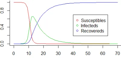
𝟏, the infection occurs and spreads. On the other hand, if 𝑹𝟎 𝟏, there is convergence of the disease as shown in the figure 2. Therefore 𝑹𝟎
𝟏 is a propagation threshold [16, 17].
Figure 2: Simulation of the stochastic SIR epi-demiology model (𝛽 1.4247, 𝛾 0.14286).
4581 2.2 The Social Network Model: Smallworld
Complex networks are present in many domains: biology, sociology, psychology, computer science, etc. We use complex networks to considerate interactions that allow the transmission of infectious diseases between individuals. Such network scan predicts the outcome of an epidemic and thus helps to test and improve public health policies. A social network can be defined as:” a group of persons or groups of people possessing patterns of contacts or interactions between them” [18]. It’s on the basis of this type of network that the modelling of the real world was introduced empirically through the Milgram experiment [19, 20].
The small-world effect is now observed on many networks coming from the real world. Several works are interested in the study of structural properties to reveal characteristics of the nodes or the structure. In the Small World graphs, two measures must be identified:
the average length of the shortest path connecting two nodes of the graph (average path length), making it possible to measure the overall accessibility of the graph;
cohesion (clustering coefficient), making it possible to measure the probability that two nodes connected to a third are connected to each other, which implies the constitution of the cliques within the network
The network assumes that the presence or absenceof an edge between two nodes is independentof the presence or absence of another edge, sothat each edge can be considered to have an independent probability P. The number of edges connected to any particular node is called the degree k of that node, and has a probability distribution Pk [21] given by:
𝑷𝒌 𝑵
𝒌 𝑷𝒌 𝟏 𝑷 𝑵 𝒌
And the average degree distribution of small world network 〈𝒌〉:
〈𝒌〉 𝒌 𝑷𝒌
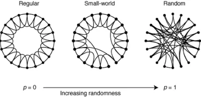
[image:3.612.326.528.183.281.2]The constitution of the Small World model starts with a regular ring network, and then a number of additional nodes is added to the middle of the network that is connected to a large number of sites (Nodes) randomly selected on the main regular network. Figure 3 represents the construction of a small world network.
Figure 3: Illustration Of Different Classes Of Networks [22].
In order to model social contacts between hu-man populations, we build a Small World net-work by representing individuals through nodes and social relationships through links. Formally, a network is described by a graph 𝐺 𝑉, 𝐸 consisting of a set of vertices V (also called nodes) where𝑉 𝑖 ∈ 𝑁 and aset E of links (also called edges) where𝐸
𝑖, 𝑗 /𝑖, 𝑗 ∈ 𝑉 hence i: source node and j:
tar-get node.
The degree of a node i, represents the neighbors of the node in an unoriented graph denoted 𝒌 𝒊 . It is the number of links between the node l and the other nodes of the graph, hence 𝒌 𝒊
𝒋/ 𝒊, 𝒋 ∈ 𝑬 . We denote by 𝑻 𝒕𝟎, 𝒕𝟏, … , 𝒕𝒎 ,
the time sequence as the disease is transmitted,
and 𝑮 𝑮𝒕𝟎, 𝑮𝒕𝟏, … , 𝑮𝒕𝒎 the network
sequence, where each element represents the network state at time t. V is a set of individuals, and Ei j is the set of edges present in the graph at
time t.
3. ALGORITHMS
3.1 Definition Of Assumptions
In order to develop our model, we have to put forward some hypotheses:
The population size is N, assumed to be fixed;
4582 At each instant t, the population is
divided into three classes: 𝑆 𝑡 : set of susceptible individuals,𝐼 𝑡 : set of infected individuals and 𝑅 𝑡 : set of recovered individuals;
An infected individual can no longer become susceptible again.
3.2 Sw Network Generation
The proposed process is based on the construction of the Small-World network, that involves two main stages. The construction of a regular ring
network and the reconnection of the edges of the graph (network).
Build a regular ring network
We begin by creating a regular ring network
𝐺 𝑡 with N nodes (the total number of nodes
representing the total population) and k edges per node (k denotes the degree of a node or the number of its neighbors). We assume that the contact networks to be constructed will be unoriented graphs in such a way that the link between two nodes (source, target) is the same as (target, source). We set up an algorithm to build the regular network:
Algorithm 1: Building the regular ring network Input: N, k
Output: G(t) Begin
for k < (N-1)/2 do if N is even then
if k is even then
for i = 1 to N do
for j = 1 to k/2 do d = i + k/2 if d > N then
Connect node[i] with node[d-N] else
Connect node[i] with node[d] end
end end
else
for i = 1 to N do
for j = 0 to (k-1)/2 do d = i + N/2-j if d > N then
Connect node[i] with node[d-N] else
Connect node[i] with node[d] end
end end
end else
for i = 1 to N do
for j = 0 to (k-1)/2 do d = i + j if d > N then
Connect node[i] with node[d-N] else
Connect node[i] with node[d] end
end end
4583 Return G(t)
END
Reconnect the edges with random probability 𝑃
the process that follows the algorithm is:
In the graph G (t), some edges are randomly reconnected with a probability of reconnection
𝑃 byreplacing 𝑁𝑜𝑑𝑒 𝑖 , 𝑁𝑜𝑑𝑒 𝑗 by
𝑁𝑜𝑑𝑒 𝑖 , 𝑁𝑜𝑑𝑒 𝑚 to avoid loops and duplicate
link. This construction allows us to switch
between the regular network 𝑃 0 , the random network 𝑃 1, and the intermediate network
0 𝑃 1 as the Small World network.
Algorithm 2: Connect the edges randomly with a probability (P) Input: G(t), k, P
Output: G(t +1) Begin
for i = 0 to N do
for j = (i+1) to i+k/2 do if j > N then
j = j - N end
Chance =Uniform random variable between 0 and 1 if P > Chance then
Node[m] chosen uniformly randomly Disconnect Node[i] and Node[j] Connect Node[i] and Node[m] end
end end
G(t) Envolves G(t +1) END
3.3 Proposed Model
In this section we combine the Small world network with the SIR model. During the disease, Individuals can have three states:
s(t): Rate of susceptible people in the population with s(t)= S(t)/N
i(t): Rate of infected people in the population with i(t)= I(t)/N
r(t): Rate of recovered people in the population with r(t)= R(t)/N
⎩ ⎪ ⎨ ⎪
⎧ 𝑑𝑠 𝑡 /𝑑𝑡 𝛽𝑁𝑠 𝑡 𝑖 𝑡 𝑑𝑖 𝑡 /𝑑𝑡 𝛽𝑁𝑠 𝑡 𝑖 𝑡 𝛾𝑖 𝑡
𝑑𝑟 𝑡 /𝑑𝑡 𝛾𝑖 𝑡
The term βNs(t) implies that all the infectious can contact all the susceptibles, in other words the graph modelling the population is completely connected. However, in the Small world complex
network [22], of which each node has 〈𝑘〉links onthe average, the assumption of complete connectionseems unreasonable. Hence the interest of replacingthe term βNs(t) with 𝛽〈𝑘〉𝑠 𝑡 , where
〈𝑘〉 is the average degree of distribution [21], that represent the average number of neighbors that an individual can have in the population. The differential equations of this model become:
⎩ ⎪ ⎨ ⎪
⎧ 𝑑𝑠 𝑡 /𝑑𝑡 𝛽〈𝑘〉𝑠 𝑡 𝑖 𝑡 𝑑𝑖 𝑡 /𝑑𝑡 𝛽〈𝑘〉𝑠 𝑡 𝑖 𝑡 𝛾𝑖 𝑡
𝑑𝑟 𝑡 /𝑑𝑡 𝛾𝑖 𝑡
The numerical method used to solve the differential equations is the Euler method based on the discretization of the variable t. The problem (2)
4584 then amounts to an iterative calculation. To perform this numerical calculation, we need:
1. The duration of the numerical calculation; 2. The initial conditions s(0), i(0) and r(0); 3. The discretization step ∆t = 1 time unit in our case.
⎩ ⎪ ⎨ ⎪
⎧ 𝑠 𝑡 1 𝑠 𝑡 𝛽〈𝑘〉𝑠 𝑡 𝑖 𝑡
𝑖 𝑡 1 𝑖 𝑡 1 𝛽〈𝑘〉𝑠 𝑡 𝛾
𝑟 𝑡 1 𝑟 𝑡 𝛾𝑖 𝑡
Algorithm 3: SIR-Small World model Input: G(t), k, 𝛽, 𝛾
Output: i(t) BEGIN Time: t t0;
i(t) = 0;
Initially: infect some nodes; While i(t) 0 do
i increases by β〈k〉s(t)i(t) with
〈𝑘〉 𝑘 𝑃
i decreases by 𝛾𝑖 𝑡 ; s decreases byβ〈k〉s(t)i(t); r increases by 𝛾𝑖 𝑡 ; t = t +1;
G(t) evolves to G(t +1); end
Return i(t) END
3.4 The Basic Reproduction Rate: R0
The dynamics of person-to-person transmission of vector transmission can be summarized by two main parameters: reproduction rate and serial or intergenerational interval [7]. A parameter of interest of the proposed model is the reproduction rate R0, which is interpreted as the average
number of new cases generated by an infectious subject in a susceptible population. This parameter is very important in the study of the spread of epidemics, it makes possible the evaluation of an infectious disease, for example, the monitoring of the evolution of virulence in case of maximization of the value of R0 and,
consequently, to predict the evolution of the epidemic over time. The more the basic reproduction number R0 increases the more the
epidemic spreads. In the case of a seasonal influenza epidemic, this parameter is measured betweenR0 = 1, and R0 = 2 [23]. To
calculate R0 we use the next generation
matrix FV-1 [24]. Mathematically the basic
reproduction number is defined as:
𝑅0 𝜌 𝐹𝑉
Where, F is the nonnegative matrix, of the new infection terms, and V is the M-matrix, of the transition terms associated with the model (2). We are interested in working only with positive orthant since the solutions are positive. The system has a unique Disease Free Equilibrium which is obtained by setting i = 0, given by:
𝐷𝐹𝐸 𝑠∗, 0,1 𝑠∗
From the system we have:
𝐹 β〈k〉s∗ and 𝑉 𝛾
Hence the basic reproduction number is given by:
𝑅 𝛽〈𝑘〉𝑠∗ 𝛾
(6)
(7) (5)
(4)
4585 In the case of R0 > 1, the introduction of an infectious agent into a susceptible population triggers an epidemic. Otherwise if R0 ≤ 1, the epidemic goes out, so the stability of the DFE. This is the famous threshold theorem, the threshold concept was used by Ross elementally in his” mosquito theorem” [25] and was developed to the famous threshold theorem of Kermackand McKendrickin 1927 [26]. In our study, we calculated the value R0 =0,352. This means that the state of equilibrium of the epidemic wave of influenza is endemic.
4. SIMULATION AND VALIDATION
4.1 Methods And Results
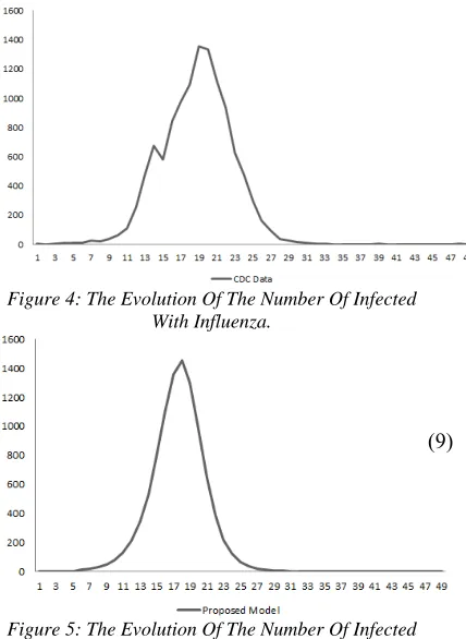
[image:7.612.92.306.415.708.2]The database used in this study is for the 2004and 2005 seasonal influenza illness in the United States. This is an epidemiological database obtained from the CDC Centers for Disease Control and Prevention. It consists of 157,759 samples that have been tested in people with influenza-like symptoms. The first week, N = 0, corresponds to the last week of September [27], as represented in figure 4.
Figure 4: The Evolution Of The Number Of Infected With Influenza.
Figure 5: The Evolution Of The Number Of Infected According To The Proposed Model.
To validate our model, we performed simulation experiments with the recommended parameters [13], figure 5. We compare the evolution of the incidence curves obtained by our model and the influenza data for the epidemic wave. A statistical analysis was applied to validate the proposed model. This is an important step in any model construction process. We used linear correlation analysis and the Kolmogorov-Smirnov test to compare observed (real) data with numerical simulations.
4.2 VALIDATION TESTS
4.2.1 Correlation
Correlation is widely used in science as a measure of the degree of linear dependency between two variables. In this work, linear correlation is used to measure the degree of similarity between the simulated data obtained by our model and the observed (real) data, Correlation coefficient= 0,88371. We find that the proposed model fits precisely the dynamic behavior of observed data used in our study.
4.2.2 The kolmogorov-smirnov test
The Kolmogorov-Smirnov test is a non-parametric matching test used to determine whether a sample follows a given law known by its continuous distribution function F(x) or whether two samples follow the same law. Indeed, it is an adjustment test to check whether the observed data are compatible with a given theoretical model. Let x1,x2,... ,xn, a sequence of n
realizations of the random variable x independent and identically distributed. We assume the following hypotheses:
H0: x follows the law of F against H1: x follows
another law ie. F = F0 against F ≠ F0.
The Kolmogorov-Smirnov test is defined by the test statistic:
𝑫𝒎𝒂𝒙 𝑺𝒖𝒑|𝑭𝒏 𝒙 𝑭𝟎 𝒙 |/𝒙 ∈ ℝ
It consists in rejecting the hypothesis H0 if
𝑫𝒎𝒂𝒙 𝑫𝒏 𝒏, 𝒂 . In other words, the larger
the test statistic D, the more likely it is to reject H0. Thus, the Kolmogorov-Smirnov test for a
4586 will test the hypothesisfor the distributions of the two sets of data to be identical, ie, both functions have the same distribution functions, which confirms the null hypothesis (H0). The statistic
test, here designated 𝑫𝒎𝒂𝒙, was the maximum deviation between the cumulative proportions of
the two functions, 𝑫𝒎𝒂𝒙
𝟎, 𝟎𝟑𝟔𝟔𝟑 𝑫𝒏 𝒏, 𝒂 𝟎, 𝟐𝟖𝟓.Indeed,
𝑫𝒎𝒂𝒙 𝟎, 𝟐𝟖𝟓, the null hypothesis (H0) is
accepted at a level of 5% confidence. Both distributions are compliant.
4.2.3 Analysis of the model
This section showshow the degree of distribution
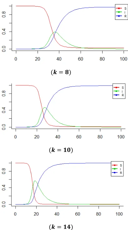
〈𝒌〉 could directlyinfluence the evolution of a disease in a social network.The following figure 6 shows the results of thesimulation of the proposed model with different k.
𝒌 𝟖
𝒌 𝟏𝟎
[image:8.612.319.530.40.231.2]𝒌 𝟏𝟒
[image:8.612.91.297.316.687.2]Figure 6: Simulation Of The SIR-Small Worldmodel With Different K.
Figure 7: Curve Of I As A Function Of K.
By comparing the above figures, we notice that the average degree distribution 〈𝒌〉 has a significant impact on the topology of the network. When the value of this factor increases, the structure of the network becomes more complex. We also observe that the epidemic spreads rapidly in densely connected groups of individuals as illustrated in figure 7. Therefore, within asocial network, the number k must be kept low because the disease spreads faster if this value of degree becomes important. Decision makers and public health professional scan simulate different epidemic scenarios using this model. This allows them to understand the mechanism of spread and to predict the final outcome of the disease by modifying the parameters of the epidemic and the state variables.
5. CONCLUSION
4587 REFERENCES
[1] Stephen R Proulx, Daniel EL Promislow, and Patrick CPhillips. Network thinking in ecology and evolution. Trends in Ecology &
Evolution, 20(6):345–353,
2005,doi:10.1016/j.tree.2005.04.004
[2] Matt J Keeling and Ken TD Eames. Networks and epidemic models. Journal of the Royal Society Interface,2(4):295–307, 2005, doi:10.1098/rsif.2005.0051
[3] K Dietz and D Schenzle. Mathematical models for infectious disease statistics. In A celebration of statistics, pages 167–204. Springer, 1985, doi:10.1007/978-1-4613-8560-88
[4] KWickwire. Mathematical models for the control of pests and infectious diseases: a survey. Theoretical population biology,11(2):182–238, 1977, doi:10.1016/0040-5809(77)90025-9
[5] Vincenzo Capasso and V Capasso. Mathematical structures of epidemic systems, volume 88. Springer, 1993
[6] LJ Allen, Fred Brauer, Pauline Van den Driessche, and Jianhong Wu. Mathematical epidemiology, volume 1945.Springer, 2008
[7] Roy MAnderson, Robert MMay, and B Anderson. Infectious diseases of humans: dynamics and control, volume 28. Wiley Online Library, 1992
[8] Robert M May. The scientific wealth of nations. Science, 275(5301):793–796, 1997,doi:10.1126/science.275.5301.793
[9] Leon Danon, Ashley P Ford, Thomas House, Chris P Jewell,Matt J Keeling, Gareth O Roberts, Joshua V Ross, and Matthew C Vernon. Networks and the epidemiology of infectious disease. Interdisciplinary perspectives on infectious
diseases, 2011, 2011,
doi:10.1155/2011/284909
[10] MM Telo da Gama and A Nunes. Epidemics in small world networks. The European Physical Journal BCondensedMatter and Complex Systems, 50(1):205–208,2006, doi:10.1140/epjb/e2006-00099-7
[11] Ming Liu and Yihong Xiao. Modeling and analysis of epidemic diffusion within small-world network. Journal of Applied
Mathematics, 2012, 2012,
doi:10.1155/2012/841531
[12] Martin Dottori and Gabriel Fabricius. Sir model on a dynamical network and the
endemic state of an infectious disease. Physica A: Statistical Mechanics and its Applications,434:25–35,
2015,doi:10.1016/j.physa.2015.04.007
[13] Gadi Fibich. Bass-sir model for diffusion of new productsin social networks. Physical
Review E, 94(3):032305,
2016,doi:10.1103/PhysRevE.94.032305
[14] PanpitSuwangool. Infectious diseases, 2-volume set 4th edition. THE BANGKOK MEDICAL JOURNAL, 13(1), 2017
[15] Younsi, Fatima-Zohra, et al. "SEIR-SW, simulation model of influenza spread based on the small world network." Tsinghua Science and Technology 20.5, 460-473, doi: 10.1109/TST.2015.7297745
[16] TeruhikoYoneyama, Sanmay Das, and Mukkai Krishnamoorthy.A hybrid model for disease spread and an application to the sars pandemic. arXiv preprint arXiv:1007.4523,
2010,doi:10.18564/jasss.1782
[17] RM Anderson and RM May. Infectious diseases of humans.oxford university press, oxford. 757p, 1991
[18] Alain Degenne and Michel Forse. Les reseaux sociaux. 2004, ISBN:978-2200266622
[19] Stanley Milgram. Behavioral study of obedience. The Journal of abnormal and social psychology, 67(4):371, 1963,doi:10.1037/h0040525
[20] Yan W Chen, Lu F Zhang, and Jian P Huang. The watts–strogatz network model developed by including degree distribution: theory and computer simulation. Journal of Physics A: Mathematical and Theoretical, 40(29):8237, 2007,doi:10.1088/1751-8113/40/29/003
[21] Mark EJ Newman, Steven H Strogatz, and Duncan JWatts. Random graphs with arbitrary degree distributions and their applications. Physical review E, 64(2):026118,
2001,doi:10.1103/PhysRevE.64.026118
[22] Duncan J Watts and Steven H Strogatz. Collective dynamics of small-world networks. nature, 393(6684):440–442, 1998,doi:10.1038/30918
4588 populations. Journal of mathematical biology,28(4):365–382, 1990, doi:10.1007/BF00178324
[24] Pauline Van den Driessche and James Watmough. Reproduction numbers and sub-threshold endemic equilibria for compartmental models of disease transmission. Mathematical biosciences, 180(1):29–48, 2002, doi:10.1016/S0025-5564(02)00108-6
[25] Ronald Ross. The prevention of malaria. John Murray; London,1911
[26] William O Kermack and Anderson G McKendrick. A contribution to the mathematical theory of epidemics. In Proceedings of the Royal Society of London A: mathematical, physical and engineering sciences, volume 115, pages 700–721. The
Royal Society, 1927,
doi:10.1098/rspa.1927.0118
[27] Centers for disease control and prevention.
Accessed: