www.hydrol-earth-syst-sci.net/19/2409/2015/ doi:10.5194/hess-19-2409-2015
© Author(s) 2015. CC Attribution 3.0 License.
Multi-objective parameter optimization of common
land model using adaptive surrogate modeling
W. Gong1,2, Q. Duan1,2, J. Li1,2, C. Wang1,2, Z. Di1,2, Y. Dai1,2, A. Ye1,2, and C. Miao1,2
1College of Global Change and Earth System Science (GCESS), Beijing Normal University, Beijing 100875, China 2Joint Center for Global Change Studies, Beijing 100875, China
Correspondence to: W. Gong ([email protected])
Received: 30 April 2014 – Published in Hydrol. Earth Syst. Sci. Discuss.: 24 June 2014 Revised: 5 March 2015 – Accepted: 10 April 2015 – Published: 21 May 2015
Abstract. Parameter specification usually has significant in-fluence on the performance of land surface models (LSMs). However, estimating the parameters properly is a challeng-ing task due to the followchalleng-ing reasons: (1) LSMs usually have too many adjustable parameters (20 to 100 or even more), leading to the curse of dimensionality in the param-eter input space; (2) LSMs usually have many output vari-ables involving water/energy/carbon cycles, so that calibrat-ing LSMs is actually a multi-objective optimization problem; (3) Regional LSMs are expensive to run, while conventional multi-objective optimization methods need a large number of model runs (typically ∼105–106). It makes parameter opti-mization computationally prohibitive. An uncertainty quan-tification framework was developed to meet the aforemen-tioned challenges, which include the following steps: (1) us-ing parameter screenus-ing to reduce the number of adjustable parameters, (2) using surrogate models to emulate the re-sponses of dynamic models to the variation of adjustable pa-rameters, (3) using an adaptive strategy to improve the effi-ciency of surrogate modeling-based optimization; (4) using a weighting function to transfer multi-objective optimization to single-objective optimization. In this study, we demon-strate the uncertainty quantification framework on a single column application of a LSM – the Common Land Model (CoLM), and evaluate the effectiveness and efficiency of the proposed framework. The result indicate that this framework can efficiently achieve optimal parameters in a more effective way. Moreover, this result implies the possibility of calibrat-ing other large complex dynamic models, such as regional-scale LSMs, atmospheric models and climate models.
1 Introduction
Land surface models (LSMs), which offer land surface boundary condition for atmospheric models and climate models, are widely used in weather and climate forecast-ing. They are also a tool for studying the impacts of climate change and human activities on our environment. Parameters of LSMs usually have significant influence on their simula-tion and forecasting capability. It has been shown that tuning even one or two parameters may significantly enhance the simulation ability of a LSM (e.g., Henderson-Sellers et al., 1996; Liang et al., 1998; Lohmann et al., 1998; Wood et al., 1998). How to specify the parameters in a LSM properly, however, remains a very challenging task because the LSM parameters are usually not directly measurable at the scale of model applications.
Automatic optimization approaches have been frequently used in calibrating the parameters of hydrological models. There is a plethora of optimization approaches available, in-cluding single-objective optimization methods such as the Shuffled Complex Evolution Metropolis, University of Ari-zona (SCE-UA) (Duan et al., 1992, 1993, 1994), the Shuf-fled Complex Evolution Metropolis, University of Arizona (SCEM-UA) (Vrugt et al., 2003a), genetic algorithm (Wang, 1991) and multi-objective optimization methods such as the Multiple-Objective Complex Optimization Method, Univer-sity of Arizona (MOCOM-UA) (Boyle et al., 2000; Boyle, 2000; Gupta et al., 1998; Yapo et al., 1998) and the Multi-Objective Shuffled Complex Evolution Metropolis, Univer-sity of Arizona (MOSCEM-UA) (Vrugt et al., 2003b).
LSM community, especially for large spatial-scale applica-tions. The major obstacles to calibrating LSMs over a large spatial scale are (1) there are too many parameters to cal-ibrate, namely, the curse of dimensionality in parameters; (2) dimensionality of the output space is too high (i.e., many processes such as water/energy/carbon cycles are simulated simultaneously); (3) conventional optimization methods, es-pecially the multi-objective approach, need a large number (∼105–106) of model runs; and the large complex dynamic system models such LSMs are usually expensive to run (i.e., costing many CPU hours). There have been numerous at-tempts to use multi-objective optimization to calibrate the parameters of LSMs and significant improvement in LSM performance measures as a result of optimization have been reported (e.g., Bastidas et al., 1999; Gupta et al., 1999; Lep-lastrier et al., 2002; Xia et al., 2002). However, the optimiza-tion efforts in the past were usually limited to cases involv-ing only point or limited spatial domain-scale applications of LSMs (Liu et al., 2003, 2004, 2005). To take a multi-objective optimization approach to the calibration of LSM parameters for large-scale applications, the key is to reduce the number of model runs to an appropriate level that we can afford.
Surrogate-based optimization is one of the most com-monly used approaches to optimizing large complex dynamic models. Several books and literature reviews have described the advances of surrogate-based optimization in recent years (e.g., Jones, 2001; Ong et al., 2005; Jin, 2011; Koziel and Leifsson, 2013; Wang et al., 2014). Surrogate-based opti-mization has been applied to economics, robotics, chemistry, physics, civil and environmental engineering, computational fluid dynamics, aerospace designs, etc. (Gorissen, 2010). On the development of surrogate-based optimization, Jones et al. (1998) proposed EGO (effective global optimizer) for pensive models using design and analysis of computer ex-periments (DACE) stochastic process model, namely, krig-ing interpolation method, as surrogate model. Castelletti et al. (2010) developed a multi-objective optimization method for water quality management using radial basis function (RBF), inverse distance weighted andn-dimensional linear interpolator as surrogates. Loshchilov et al. (2010) investi-gated the use of the ranked-based support vector machine (SVM) and demonstrated that for surrogate-based optimiza-tion capturing the relative value of the objective funcoptimiza-tions is more important than reducing the absolute fitting error. Pilát and Neruda (2013) developed a surrogate model selec-tor for multi-objective surrogate-assisted optimization. In hy-drology and water resources, Razavi et al. (2012) has sum-marized recent applications, advantages and existing prob-lems. Wang et al. (2014) evaluated the influence of ini-tial sampling and adaptive sampling methods for surrogate-assisted optimization of a simple hydrological model, the Sacramento Soil Moisture Accounting (SAC-SMA) model. Song et al. (2012) optimized the parameter of a distributed hydrological model – distributed time-variant gain model’s
(DTVGM) – with an SCE-UA algorithm using the Multi-variate Adaptive Regression Splines (MARS) method (Fried-man, 1991) as surrogate.
In our recent works, we proposed a framework that can potentially reduce the number of model runs needed for pa-rameter calibration of large complex system models (Wang et al., 2014). This framework involves the following steps: (1) a parameter screening step using global sensitivity analy-sis to identify the most sensitive parameters to be included in the optimization; (2) surrogate modeling that can emulate the response surface of the dynamic system model to the change in parameter values; (3) an adaptive sampling strategy to im-prove the efficiency of the surrogate model construction; and (4) a multi-objective optimization step to optimize the most sensitive parameters of the dynamic system model. In this paper, we will illustrate this parametric uncertainty quantifi-cation framework with the Common Land Model (CoLM), a widely used, physically based LSM developed by Dai et al. (2003, 2004) and Ji and Dai (2010). The work related to parameter screening and surrogate modeling-based optimiza-tion (adaptive surrogate model-based optimizaoptimiza-tion strategy – ASMO) method for single objective has already been pub-lished (Li et al., 2013; Wang et al., 2014). This paper will emphasize the analysis of different surrogate model construc-tion methods and multi-objective optimizaconstruc-tion methods and results.
This paper contains the following parts: Sect. 2 introduces the basic information of CoLM, the study area and data set, the adjustable parameters and the output variables to be an-alyzed; Sect. 3 presents an inter-comparison of five surro-gate modeling methods, and discusses how many model runs would be sufficient to build a surrogate model for optimiza-tion; Sect. 4 carries out single and multiple objective opti-mization using an ASMO strategy; Sect. 5 provides the dis-cussion and conclusions.
2 Experiment setup 2.1 Model and parameters
Table 1. Adjustable parameters and their categories, meanings and ranges.
Num Para Units Category Physical meaning Feasible range
P1 dewmx canopy maximum dew ponding of leaf area [0.05, 0.15]
P2 hksati mm s−1 soil maximum hydraulic conductivity [0.001, 1]
P3 porsl – soil porosity [0.25, 0.75]
P4 phi0 mm soil minimum soil suction [50, 500]
P5 wtfact soil fraction of shallow groundwater area [0.15, 0.45]
P6 bsw – soil Clapp and Hornbergerbparameter [2.5, 7.5]
P7 wimp soil water impermeable if porosity less than wimp [0.01, 0.1]
P8 zlnd m soil roughness length for soil surface [0.005, 0.015]
P9 pondmx mm soil maximum ponding depth for soil surface [5, 15]
P10 csoilc – soil drag coefficient for soil under canopy [0.002, 0.006]
P11 zsno m snow roughness length for snow [0.0012, 0.0036]
P12 capr soil tuning factor of soil surface temperature [0.17, 0.51]
P13 cnfac canopy Crank Nicholson factor [0.25, 0.5]
P14 slti canopy slope of low temperature inhibition function [0.1, 0.3]
P15 hlti canopy 1/2 point of low temperature inhibition function [278, 288]
P16 shti canopy slope of high temperature inhibition function [0.15, 0.45]
P17 sqrtdi m−0.5 canopy the inverse of square root of leaf dimension [2.5, 7.5]
P18 effcon mol CO2mol−1quanta canopy quantum efficiency of vegetation photosynthesis [0.035, 0.35]
P19 vmax25 mol CO2m−2s canopy maximum carboxylation rate at 25◦ [10−6, 200−6]
P20 hhti canopy 1/2 point of high temperature inhibition function [305, 315]
P21 trda canopy temperature coefficient of conductance–photosynthesis model [0.65, 1.95]
P22 trdm canopy temperature coefficient of conductance–photosynthesis model [300, 350]
P23 trop canopy temperature coefficient of conductance–photosynthesis model [250, 300]
P24 gradm canopy slope of conductance–photosynthesis model [4, 9]
P25 binter canopy intercept of conductance–photosynthesis model [0.01, 0.04]
P26 extkn canopy coefficient of leaf nitrogen allocation [0.5, 0.75]
P27 chil canopy leaf angle distribution factor [−0.3, 0.1]
P28 ref(1,1) canopy Visible (VIS) reflectance of living leaf [0.07, 0.105]
P29 ref(1,2) canopy VIS reflectance of dead leaf [0.16, 0.36]
P30 ref(2,1) canopy near-infrared (NIR) reflectance of living leaf [0.35, 0.58]
P31 ref(2,2) canopy NIR reflectance of dead leaf [0.39, 0.58]
P32 tran(1,1) canopy VIS transmittance of living leaf [0.04, 0.08]
P33 tran(1,2) canopy VIS transmittance of dead leaf [0.1, 0.3]
P34 tran(2,1) canopy NIR transmittance of living leaf [0.1, 0.3]
P35 tran(2,2) canopy NIR transmittance of dead leaf [0.3, 0.5]
P36 z0m m canopy aerodynamic roughness length [0.05, 0.3]
P37 ssi snow irreducible water saturation of snow [0.03, 0.04]
P38 smpmax mm soil wilting point potential [−2.e5,−1.e5]
P39 smpmin mm soil restriction for min of soil potential [−1.e8,−9.e7]
P40 trsmx0 mm s−1 canopy maximum transpiration for vegetation [1.e-4, 1. e-2]
This study considers six output variables simulated by CoLM: sensible heat, latent heat, upward long-wave radia-tion, net radiaradia-tion, soil temperature and soil moisture. The normalized root mean squared error (NRMSE) is used as the objective function in our analysis:
NRMSEi= s
N P
j=1
yi,jsim−yi,jobs
2
N P
j=1
yi,jobs
, (1)
whereiis the index of output variables,j is the index of time step, N is the total number of observations, yi,jsim andyi,jobs
are the simulated and observed values, respectively.
Objec-tive functions represent the performance of model simulation and a smaller objective function means better performance. 2.2 Study area and data sets
The study area and associated data sets are from the Heihe river basin, the same as in Li et al. (2013). The Heihe river basin, which is located between 96◦420–102◦000E and
sta-tion located at the upstream region of the Heihe river basin. Its geographic coordinate is 100◦280E, 38◦030N, altitude is
3032.8 m above sea level and the land cover type is alpine steppe.
The forcing data used include downward shortwave and long-wave radiation, precipitation, air temperature, relative humidity, air pressure and wind speed (Hu et al., 2003); the observation data used to validate the simulation of CoLM include: sensible heat, latent heat, upward long-wave radia-tion, net radiaradia-tion, soil temperature and soil moisture. The soil temperature and moisture were measured at depth 10, 20, 40 and 80 cm. In CoLM, the soil is divided into 10 layers and the simulated soil temperature and soil moisture are lin-early interpolated to the measured depth. Currently, we have 2 years of observation data. The data from year 2008 was used for spin-up and that of 2009 was used for parameter screening, surrogate modeling and optimization. The simu-lation time step is set to 30 min and the simusimu-lation outputs are averaged to 3 h in order to compare with the observation data.
3 Comparison of surrogate models
After the sensitive parameters are identified using global sen-sitivity methods (see Li et al., 2013), the next step is to cal-ibrate the sensitive parameters through multi-objective opti-mization. Since the calibration of CoLM in real-world appli-cations can be very expensive, we aim to establish a surro-gate model to represent the response surface of the dynamic CoLM. The surrogate model, also called response surface, meta-model, statistical emulator, is a statistical model that describes the response of output variable to the variation of input variables. Because the surrogate model only consid-ers the statistical relationship between input and output, it is usually much cheaper to run than the original large com-plex dynamic model (“original model” for short). Parameter optimization usually needs thousands, or even up to millions of model runs. It will be impossible to calibrate large com-plex dynamic models if running the original dynamic model is too time-consuming. If we can do parameter optimization with a surrogate model instead of an original model, the time of running the original model will be dramatically reduced, making it possible to calibrate the large complex dynamic models, such as LSMs, atmospheric models, or even global climate models. However, optimization based on surrogate models can be a challenging task because the response sur-face might be very bumpy and has many local optima. Razavi et al. (2012) gave a comprehensive review of the surrogate modeling methods and applications in water resources, and discussed the pitfalls of surrogate modeling as well.
[image:4.612.309.544.96.177.2]In this research, we first compared five different surrogate models: multivariate adaptive regression spline (MARS), Gaussian process regression (GPR), Random Forest (RF), support vector machine (SVM), and artificial neural network
Table 2. Screened parameters of CoLM in A’rou Station (Li et.al.,
2013).
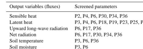
Output variables (fluxes) Screened parameters
Sensible heat P2, P4, P6, P30, P34, P36 Latent heat P3, P4, P6, P18, P19, P23, P25, P36 Upward long-wave radiation P6, P17, P36
Net radiation P6, P17, P30, P34, P36 Soil temperature P3, P6, P36
Soil moisture P3, P6
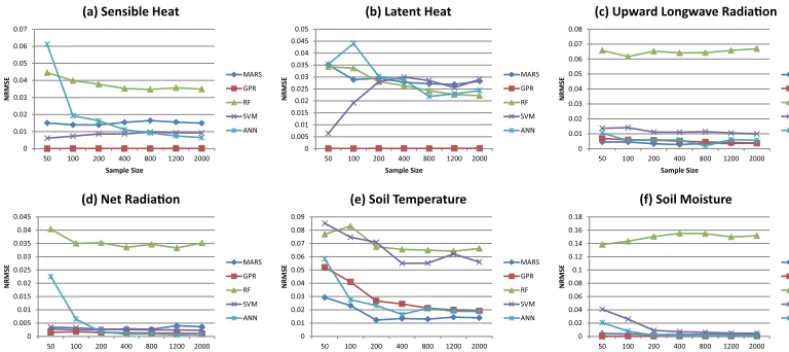
(ANN). A brief introduction of these methods is provided in the Appendix. To build a surrogate, we need to choose a sam-pling method first. The samsam-pling method used in this study is the Latin hypercube (LH) Sampling (McKay et al., 1979). The sample sizes are set to 50, 100, 200, 400, 800, 1200, and 2000. The inter-comparison results are shown in Figs. 1 and 2, in which thexaxis is the sample size, andyaxis is the NRMSE (i.e., the ratio of the root mean square error (RMSE) of the simulation model and the surrogate model). Figure 1 shows the error of the training set, namely, the NRMSE be-tween the outputs predicted by the surrogate model and the outputs of the training samples, and Fig. 2 shows the NRMSE of the testing set. Since every sample set of each size was in-dependently generated, we use the 2000 points set to test 50, 100, 200, 400, 800 and 1200 points set, and use the 1200 one to test the 2000 one. For each output variable, we only construct surrogate models for the most sensitive parameters based on the screening results obtained by Li (2012) and Li et al. (2013) (see Table 2).
As shown in Fig. 1, for some cases, such as upward long-wave radiation, the fitting ability of the training set does not change significantly with sample size, but for soil mois-ture, larger sample size leads to better fitted surrogate mod-els. Such phenomenon indicated that the specific features of the response surfaces have significant influence on the fit-ting ability, and good surrogate models must have the ability to adapt to those features. As shown in Fig. 1, GPR has the best fitting ability for almost every case except soil tempera-ture. As described in Appendix 2, the hyper-parameters used by GPR can be adaptively determined using the maximum marginal likelihood method.
vari-0 0.01 0.02 0.03 0.04 0.05 0.06 0.07
50 100 200 400 800 1200 2000
NRMSE
Sample Size
(a) Sensible Heat
MARS GPR RF SVM ANN 0 0.005 0.01 0.015 0.02 0.025 0.03 0.035 0.04 0.045 0.05
50 100 200 400 800 1200 2000
NRMSE
Sample Size
(b) Latent Heat
MARS GPR RF SVM ANN 0 0.01 0.02 0.03 0.04 0.05 0.06 0.07 0.08
50 100 200 400 800 1200 2000
NRMSE
Sample Size
(c) Upward Longwave Radiaon
MARS GPR RF SVM ANN 0 0.005 0.01 0.015 0.02 0.025 0.03 0.035 0.04 0.045
50 100 200 400 800 1200 2000
NRMSE
Sample Size
(d) Net Radiaon
MARS GPR RF SVM ANN 0 0.01 0.02 0.03 0.04 0.05 0.06 0.07 0.08 0.09
50 100 200 400 800 1200 2000
NRMSE
Sample Size
(e) Soil Temperature
MARS GPR RF SVM ANN 0 0.02 0.04 0.06 0.08 0.1 0.12 0.14 0.16 0.18
50 100 200 400 800 1200 2000
NRMSE
Sample Size
(f) Soil Moisture
[image:5.612.101.496.66.242.2]MARS GPR RF SVM ANN
Figure 1. Inter-comparison of five surrogate modeling methods: error of training set.
0 0.01 0.02 0.03 0.04 0.05 0.06 0.07 0.08 0.09
50 100 200 400 800 1200 2000
NRMSE
Sample Size (a) Sensible Heat
MARS GPR RF SVM ANN 0 0.01 0.02 0.03 0.04 0.05 0.06 0.07 0.08 0.09
50 100 200 400 800 1200 2000
NRMSE
Sample Size (b) Latent Heat
MARS GPR RF SVM ANN 0 0.01 0.02 0.03 0.04 0.05 0.06
50 100 200 400 800 1200 2000
NRMS
E
Sample Size
(c) Upward Longwave Radiaon
MARS GPR RF SVM ANN 0 0.005 0.01 0.015 0.02 0.025 0.03 0.035 0.04 0.045 0.05
50 100 200 400 800 1200 2000
NRMSE
Sample Size (d) Net Radiaon
MARS GPR RF SVM ANN 0 0.02 0.04 0.06 0.08 0.1 0.12 0.14
50 100 200 400 800 1200 2000
NRMSE
Sample Size (e) Soil Temperature
MARS GPR RF SVM ANN 0 0.01 0.02 0.03 0.04 0.05 0.06 0.07 0.08 0.09
50 100 200 400 800 1200 2000
NRMSE
Sample Size (f) Soil Moisture
[image:5.612.100.495.278.451.2]MARS GPR RF SVM ANN
Figure 2. Inter-comparison of five surrogate modeling methods: error of testing set.
ables are different. For net radiation, soil temperature and soil moisture, the fitting error decreases to nearly 0 if the sam-pling points are more than 200; while for sensible heat, latent heat and upward long-wave radiation, the marginal benefit of adding more points is still significant beyond more than 200 sample points. Since the GPR method can consistently give the best performance for all six output variables, we choose GPR in the multi-objective optimization analysis presented later.
4 Optimization
4.1 Single-objective optimization
Before we conduct multi-objective optimization, we first car-ried out single-objective optimization for each output vari-able using the GPR surrogate model. The SCE method (Duan et al., 1992, 1993, 1994) is used to find the optima of the
surrogate models. In order to figure out how many sample points are sufficient to construct a surrogate model for opti-mization, different sample sizes (i.e., 50, 100, 200, 400, 800, 1200, and 2000) are experimented. To evaluate the optimiza-tion results based on the surrogate model, we also set up two control cases: (1) no optimization using the default param-eters as specified in CoLM, and (2) optimization using the original CoLM (i.e., no surrogate model is used). The second case is referred to as “direct optimization”. The control cases are used to confirm the following hypotheses: (1) parameter optimization can indeed enhance the performance of CoLM; (2) optimization using the surrogate model can achieve simi-lar optimization results as using the original model, but with fewer model runs.
0 0.2 0.4 0.6 0.8 1
P2 P4 P6 P17 P30 P34 P36
(a) Sensible Heat
0 0.2 0.4 0.6 0.8 1
P3 P4 P6 P18 P19 P23 P25 P36
Normalized parameter
0 0.2 0.4 0.6 0.8 1
P6 P17 P36
0 0.2 0.4 0.6 0.8 1
P6 P17 P30 P34 P36
Normalized parameter
(b) Latent Heat (c) Upward Longwave Radiation
(d) Net Radiation
0 0.2 0.4 0.6 0.8 1
P3 P6 P36
(e) Soil Temperature
0 0.2 0.4 0.6 0.8 1
P3 P6
LH50
LH100
LH200
LH400
LH800
LH1200
LH2000 (f) Soil Moisture
[image:6.612.97.488.65.252.2]SCE
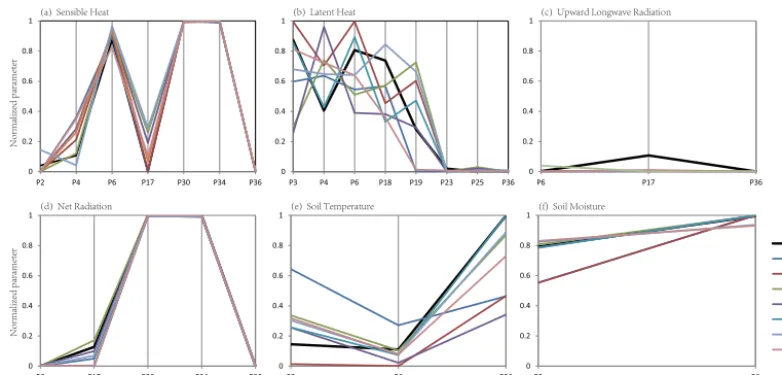
Figure 3. Single-objective optimization result: optimal parameters.
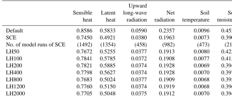
using the original CoLM, and other lines are optimal param-eters given by surrogate models created with different sam-ple sizes. Table 3 summarizes the optimized NRMSE values of all surrogate model-based optimization runs with differ-ent sample sizes, as well as the control cases. The numbers of original model runs that SCE takes are also listed in the parentheses.
The optimization results reveal that (1) parameter opti-mization can significantly improve the simulation ability of CoLM for all output variables. (2) For sensible heat, upward long-wave radiation, net radiation, soil moisture, the optimal parameters obtained by surrogate model optimization runs are very similar to those obtained by direct optimization. The optimal parameters obtained for different sample sizes are also close to each other. For latent heat and soil temperature, however, the optimal parameters given by surrogate model optimization and direct optimization are significantly differ-ent. The discrepancy between the results with different sam-ple sizes is also significant, comparing to the previous four outputs. (3) Surprisingly, for four of the outputs, namely, some variables (e.g., sensible heat, upward long-wave ra-diation, net radiation and soil moisture), sample size does not have significant influence on the optimization results. As shown in Table 3, even a surrogate model constructed with 50 samples is similar to the one constructed with 2000 sam-ples and with the direct optimization. For soil temperature, 200 samples are sufficient, and for latent heat, more than 400 samples are enough. Interestingly, the LH50’s optimization result for sensible heat is even smaller than that of LH2000. This is because LH sampling is random and the LH50 sam-pling may have produced a sample point very close to the global optimum, while the best sample point of the LH2000 sampling may be further away from the global optimum. Consequently, the number of samples required for surrogate-based optimization varies for different outputs because of the
randomness of sampling designs, and the complexity of re-sponse surfaces. A more complex surface needs more sam-ple points to build an effective surrogate model, compared to a simple surface. Even so, this result is very encouraging in that with the help of surrogate models we can possibly reduce the number of model runs required by optimization down to hundreds of times. (4) The number of original model runs that SCE takes before convergence is also listed in Table 3. The result indicated that SCE can get better, or similar op-timal NRMSE, but the number of model runs is larger than that using the surrogate model. If the original dynamic model costs too much CPU time to run, surrogate-based optimiza-tion can be more efficient than the SCE. (5) Different output variables require different optimal parameters, indicating the necessity of multi-objective optimization. For example, P6, the Clapp and Hornberger “b” parameter, is sensitive to many outputs. For sensible heat, latent heat and soil moisture, the optimal value of P6 is high, while for upward long-wave ra-diation, net radiation and soil temperature, the optimal value of P6 is low. In order to balance the performance of all out-put variables, it is necessary to choose a compromised value for P6. Multi-objective optimization is an approach that can provide such a compromised optimal parameter that balances the requirements of many output variables.
4.2 Multi-objective optimization
Table 3. The NRMSE between simulated and observed outputs after single-objective optimization.
Upward
Sensible Latent long-wave Net Soil Soil
heat heat radiation radiation temperature moisture
Default 0.8586 0.5833 0.0590 0.2357 0.0096 0.4527
SCE 0.7450 0.4921 0.0380 0.1963 0.0073 0.3900
No. of model runs of SCE (1492) (1354) (458) (982) (473) (210)
LH50 0.7672 0.5255 0.0377 0.1913 0.0080 0.4222
LH100 0.7841 0.5785 0.0372 0.1908 0.0077 0.4130
LH200 0.7821 0.5885 0.0374 0.1928 0.0069 0.3947
LH400 0.7798 0.5627 0.0374 0.1928 0.0070 0.3971
LH800 0.7683 0.5024 0.0377 0.1909 0.0068 0.3956
LH1200 0.7760 0.5150 0.0374 0.1919 0.0068 0.3962
LH2000 0.7705 0.5048 0.0375 0.1912 0.0070 0.3946
should be compatible with surrogate model optimization; (2) for practical reasons, it should provide a single best pa-rameter set instead of a full Pareto optimum set with many non-dominated parameter sets. The Pareto optimal set usu-ally contains hundreds of points, but for large complex dy-namic models such as regional or global LSMs, it is gener-ally impractical, and also unnecessary to run the model in an ensemble mode with hundreds of model runs. For regional or global LSMs coupled with atmospheric models, providing only one parameter set that has good simulation ability for most outputs is a more economical and convenient choice.
In multi-objective optimization, there have been many methods that can transform multiple objectives to single ob-jective. Among them, the weighting function-based method is the most intuitive and widely used one. In this paper, we assign higher weights to the outputs with larger errors. In the research of Liu et al. (2005), the RMSE of each outputs were normalized by the RMSE of the default parameter set, and each normalized RMSE was assigned equal weights. Van Griensven and Meixner (2007) developed a weighting sys-tem based on Bayesian statistics to define “high-probability regions” that can give “good” results for multiple outputs. However, both of Liu et al. (2005) and van Griensven and Meixner (2007) tended to assign higher weights to the out-puts with lower RMSE, and lower weights to the outout-puts with higher RMSE. This tendency, although reasonable in the probability meaning, conflicts with our intuitive motiva-tions that we want to emphasis on the poorly simulated out-puts with large RMSE. Jackson et al. (2003) assumed Gaus-sian error in the data and model so that the outputs were in a joint Gaussian distribution, and the multi-objective “cost function” was defined on the joint Gaussian distribution of multiple outputs. In Gupta et al. (1998), a multiple weighting function method is proposed to fully describe the Pareto fron-tier, if the frontier is convex and model simulation is cheap enough. If one outputs is more important than others, a higher weight should be assigned to it. Marler and Arora (2010) reviewed the applications, conceptual significance and
pit-falls of weighting function-based optimal methods, and gave some suggestions to avoid blind use of it.
In this study, we use three weighting functions to convert the multi-objective optimization into a single-objective op-timization. Case 1: assigning more weight if the output is simulated more poorly as compared to the other outputs. The summed up objectives should have the same unit, so we use NRMSE as the objective function. The weighting function is
F =
n X
i=1
wiNRMSEi, (2)
in which the NRMSEi is the normalized root mean squared
error of each output variable that is defined in Eq. (1),wi is
the weight of each output and
n P
i=1
wi =1. Table 4 shows the
RMSE and NRMSE of CoLM using default parameterization scheme, and the weight of each output is proportional to the NRMSE. Case 2: Liu et al. (2005) normalized the RMSE of each output with the RMSE of simulation result given by default parameters. The weighting function is
F =
n X
i=1
wi
RMSEi
RMSEi,default
(3)
and assign equal weights to each normalized output. Case 3: van Griensven and Meixner (2007) defined the global optimization criterion (GOC) based on Bayesian theory for multi-objective optimization. If the number of observations of each output are the same, the GOC is defined as
F =
n X
i=1 SEi
SEi,min
, (4)
where SEi = N P
j=1
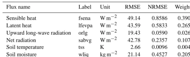
Table 4. Weights assigned to each output variables (weighting system case 1).
Flux name Label Unit RMSE NRMSE Weights
Sensible heat fsena W m−2 49.14 0.8586 0.3905
Latent heat lfevpa W m−2 43.59 0.5833 0.2653
Upward long-wave radiation orlg W m−2 19.43 0.0590 0.0268
Net radiation sabvg W m−2 42.78 0.2357 0.1072
Soil temperature tss K 2.66 0.0096 0.0044
Soil moisture wliq kg m−2 21.14 0.4527 0.2059
In order to use the information offered by the surrogate model more effectively, we developed an adaptive surrogate modeling-based optimization method called ASMO (Wang et al., 2014). The major steps of ASMO are as follows: (1) construct a surrogate model with initial samples, and find the optimal parameter of the surrogate model. (2) Run the original model with this optimal parameter and get a new sample. (3) Add the new sample to the sample set and con-struct a new surrogate model, and then go back to the 1st step. The effectiveness and efficiency of ASMO have been vali-dated in Wang et al. (2014) using 6D Hartman function and a simple hydrologic model SAC-SMA. As shown in the com-parison between ASMO and SCE-UA, ASMO is more effi-cient in that it can converge with less model runs, while SCE-UA is more effective in that it can get closer to the true global optimal parameter. So making a choice between ASMO and SCE-UA is a “cost-benefit” trade-off: if the model is very cheap to run, SCE-UA is preferred because it is more effec-tive to find the global optimum; while if the model is very expensive to run, ASMO is preferred because it can find a fairly good parameter within a limited number of model runs. Such parameter set can provide only the approximate global optimum, but this approach is much cheaper than using tra-ditional approaches such as SCE-UA.
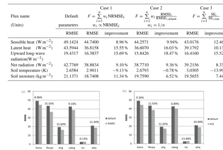
We carried out multi-objective optimization with ASMO using weighting functions defined in Eqs. (2), (3) and (4). The optimization results are shown in Table 5. The RMSEs of each case were compared with that given by the default pa-rameterization scheme, and the relative improvements were calculated. Obviously, for all three cases, all of the six out-puts were significantly improved except soil temperature. All three cases sacrificed the performance of soil temperature, but case 2 (Liu et al., 2005) decreased the least (only 0.78 %), case 3 (van Griensven and Meixner, 2007) decreased the most, and the case 1 (weights proportional to NRMSE) is the moderate one. The results indicated that all three types of weighting functions can balance the conflicting requirements of different objectives and effectively give an optimal param-eter set with ASMO algorithm. In the following studies, we only involve the moderate case (case 1).
To demonstrate the effectiveness and efficiency of surrogate-based optimization, we also carried out the di-rect optimization using SCE-UA. The weighting function
0 0.2 0.4 0.6 0.8 1
P2 P3 P4 P6 P17 P18 P19 P23 P25 P30 P34 P36
P
ara
meter Va
lu
e
(rel
a
ve
)
Parameter Index
default
ASMO
[image:8.612.311.548.204.320.2]SCE
Figure 4. Optimal value of CoLM given by multi-objective
opti-mization (comparing default parameter, optimal parameter given by ASMO and SCE-UA).
adopted was Eq. (2), and the optimization results are shown in Figs. 4 and 5. Figure 4 presents the default parameter, the optimal parameter given by ASMO and that given by SCE-UA. Figure 5 shows the improvements given by ASMO and SCE-UA comparing to the default parameters. From Fig. 5 we find that all of the outputs have improved nearly 10 % ex-cept soil temperature, and the improvements made by ASMO are similar to that by SCE-UA. The results indicated that multi-objective optimization can indeed enhance the perfor-mance of CoLM using either the ASMO or SCE-UA method. The ASMO method converged after 11 iterations, namely, the total number of model runs is 411, while the number of model runs for SCE-UA is 1000, which is the maximum model runs set for SCE-UA. Obviously, ASMO is a more efficient method compared to SCE-UA in this case.
We also used the Taylor diagram (Taylor, 2001) to com-pare the simulation results for the calibration period and the validation period (see Figs. 6 and 7). The optimization re-sults given by SCE-UA and ASMO using Eq. (2) as weight-ing function are compared against the performance of default parameterization scheme. Since only 2 years of observation data for the six output variables are available, we use the first year’s (2008) data as the warm-up period, the second year’s (2009) data as calibration period, and then use the pre-vious year’s (2008) data as the validation period. The missing records have been removed from the comparison.
Table 5. Inter-comparison of different weighting systems.
Case 1 Case 2 Case 3
Flux name Default F=
n
P
i=1
wiNRMSEi F=
n
P
i=1
wiRMSERMSEi,defaulti F=
n
P
i=1 SEi
SEi,min
(Units) parameters wi∝NRMSEi wi=1/n
RMSE RMSE improvement RMSE improvement RMSE improvement
Sensible heat (W m−2) 49.1424 44.7400 8.96 % 44.2571 9.94% 43.0176 12.46 %
Latent heat (W m−2) 43.5944 36.8158 15.55 % 36.6070 16.03 % 39.1792 10.13 %
Upward long-wave 19.4317 16.3837 15.69 % 15.8426 18.47 % 16.4160 15.52 %
radiation(W m−2)
Net radiation (W m−2) 42.7769 38.8834 9.10 % 38.7710 9.36 % 39.2156 8.33 %
Soil temperature (K) 2.6584 2.9011 −9.13 % 2.6793 −0.78 % 3.0305 −13.99 %
Soil moisture (kg m−2) 21.1371 18.7408 11.34 % 19.7590 6.52 % 19.5655 7.44 %
0 10 20 30 40 50 60
fsena lfevpa olrg sabvg tss wliq
RMS
E
default
SCE 9.36%
11.55%
11.02% 6.89%
-13.40% 10.49%
W/m2 W/m2 W/m2 W/m2 K kg/m2
0 10 20 30 40 50 60
fsena lfevpa olrg sabvg tss wliq
RMS
E
default
ASMO 8.96%
15.55%
15.69% 9.10%
-9.13% 11.34%
W/m2 W/m2 W/m2 W/m2 K kg/m2
[image:9.612.286.510.89.387.2](a) (b)
Figure 5. Comparing the improvements given by ASMO and SCE.
D in the Taylor diagram) are better than the default param-eterization scheme (Case B) except soil temperature. Even though soil temperature simulation is degraded, the correla-tion coefficients given by all three cases are higher than 0.9, indicating that this imperfection will not cause significant in-consistency in the land surface modeling. In Fig. 7, the per-formance of the validation period is shown quite similar to that in the calibration period, indicating that the optimal pa-rameters are well identified and the over-fitting problem is avoided.
The four energy fluxes (sensible/latent heat, upward long-wave radiation, net radiation) and soil surface temperature have very good performance. However, the performance of soil moisture seems unsatisfactory. The correlation coeffi-cient of soil moisture of Case B (default parameter) is less than 0, while with the help of SCE-UA and ASMO opti-mization the correlation coefficient is only slightly larger than 0. The possible reasons might be as follows: (1) the de-fault soil parameters of CoLM is derived from the soil tex-ture in the 17-category Food and Agricultural Organization State Soil Geographic (FAO-STATSGO) soil data set (Ji and Dai, 2010), which provides the top-layer (30 cm) and bottom-layer (30–100 cm) global soil textures and has a 30 s resolu-tion. The resolution and accuracy of this data set may not
perfor-(a) Sensible heat (b) Latent heat (c) Upward longwave radiation
(d) Net radiation (e) Soil temperature (f) Soil moisture
B: Defualt D: ASMO C: SCE A: Observation 20 40 60 80 0 20 0 40 0 60 0 80 1 0.99 0.95 0.9 0.8 0.7 0.6 0.5 0.4 0.3 0.2 0.1 0 Standard deviation Correla t io n C oe
f fic ient
R M S D A B CD 20 40 60 80 0 20 0 40 0 60 0 80 1 0.99 0.95 0.9 0.8 0.7 0.6 0.5 0.4 0.3 0.2 0.1 0 Standard deviation Correla t io n C oe
f fic ient
R M S D A B C D 20 40 60 80 0 20 0 40 0 60 0 80 1 0.99 0.95 0.9 0.8 0.7 0.6 0.5 0.4 0.3 0.2 0.1 0 Standard deviation Correla t io n C oe
f fic ient
R
M S
D
A BCD
50 100 150 200 0 50 0 100 0 150 0 200 1 0.99 0.95 0.9 0.8 0.7 0.6 0.5 0.4 0.3 0.2 0.1 0 Standard deviation Cor relat io
n Coe f fic
ien t R M S D A B C D 2 4 6 8 0 2 0 4 0 6 0 8 1 0.99 0.95 0.9 0.8 0.7 0.6 0.5 0.4 0.3 0.2 0.1 0 Standard deviation Cor relat io
n Coe f fic
ien t R M S D A B C D 5 10 15 20 1 0.99 0.95 0.9 0.8 0.7 0.6 0.5 0.4 0.3 0.2 0.1 0 RM SD A 0 B C D Correla t ion
Coef f icie
[image:10.612.98.452.62.301.2]nt 0 20 15 10 5 Standard deviation (W/m 2) (W/m 2) (W/m 2) (W/m 2) (kg /m 2) (K)
Figure 6. Taylor diagram of simulated fluxes during calibration period (1 January 2009 to 31 December 2009).
(a) Sensible heat (b) Latent heat (c) Upward longwave radiation
(d) Net radiation (e) Soil temperature (f) Soil moisture
B: Defualt D: ASMO C: SCE A: Observation 20 40 60 80 0 20 0 40 0 60 0 80 1 0.99 0.95 0.9 0.8 0.7 0.6 0.5 0.4 0.3 0.2 0.1 0 Standard deviation Correla t io
n Coe f fic
ien t R M S D A B CD 20 40 60 80 100 0 20 0 40 0 60 0 80 0 100 1 0.99 0.95 0.9 0.8 0.7 0.6 0.5 0.4 0.3 0.2 0.1 0 Standard deviation Correla t io n C oe
f fic ien t RM SD A B C D 20 40 60 80 0 20 0 40 0 60 0 80 1 0.99 0.95 0.9 0.8 0.7 0.6 0.5 0.4 0.3 0.2 0.1 0 Standard deviation Correla t io
n Coe f fic
ien t R M S D A
BCD
50 100 150 200 0 50 0 100 0 150 0 200 1 0.99 0.95 0.9 0.8 0.7 0.6 0.5 0.4 0.3 0.2 0.1 0 Standard deviation Correla t io n C oe
f fic ien t R M S D AB C D 2 4 6 8 0 2 0 4 0 6 0 8 1 0.99 0.95 0.9 0.8 0.7 0.6 0.5 0.4 0.3 0.2 0.1 0 Standard deviation Correla t io n C oe
f fic ien t R M S D A B C D (W/m 2) (W/m 2) (W/m 2) (W/m 2) (kg /m 2) (K) B C D 0 0 20 10 15 5 5 10 15 20 1 0.99 0.95 0.9 0.8 0.7 0.6 0.5 0.4 0.3 0.2 0.1 0 RM SD A D Cor rela
t ion C ef f ic ien t o Standard deviation C
Figure 7. Taylor diagram of simulated fluxes during validation period (here we use the warm-up period as validation period, 1 January 2008
to 31 December 2008).
mance of CoLM and cannot be mitigated by parameter opti-mization.
In the optimization results, five of the outputs were im-proved but only soil temperature became worse. In multi-objective optimization, a compromise is necessary. In this case study, soil temperature requires small P6 and large 36, which conflict with all other outputs. Consequently,
[image:10.612.100.483.337.574.2]sac-rifice of soil temperature is worthwhile because a negligible degradation of one output can lead to a significant improve-ment of all other outputs.
5 Discussion and conclusions
We have carried out multi-objective parameter optimization for a LSM (CoLM) at the Heihe river basin. Although there have been other studies, such as multi-objective calibration of hydrological models (Gupta et al., 1998; Vrugt et al., 2003b), LSMs (Gupta et al., 1999), single column land– atmosphere coupled models (Liu et al., 2005), and soil– vegetation–atmosphere transfer (SVAT) models (Pollacco et al., 2013), the novel contribution of this research lies in the significant reduction of model runs. In previous research, a typical multi-objective optimization needs∼105–106or even more model runs. For large complex dynamic models which are very expensive to run, parameter optimization is imprac-tical because of lack of computational resources. In this re-search, we managed to achieve a multi-objective optimal pa-rameter set with only 411 model runs. The performance of the optimal parameter set is similar with the one obtained by SCE-UA method using more than 1000 model runs. Such a result indicates that the proposed framework in this paper is able to provide optimal parameters more efficiently. In future work, we are going to extend the uncertainty quantification framework to other large complex dynamic models, such as regional-scale LSMs, atmospheric models and climate mod-els. We will look into testing the scalability of the screen-ing, surrogate modeling and optimization techniques on more complex models with more adjustable parameters. We will also investigate the influence of uniformity and stochastic-ity of initial sampling points, and compare the suitabilstochastic-ity of different sampling methods. In addition to examining the main and total effects of the parameters, we will also eval-uate the interactions among parameters. We will continue to improve the effectiveness, efficiency, flexibility and ro-bustness of GPR approach for surrogate modeling, and test with more complex models. Since weighting function-based multi-objective optimization methods are simple, intuitive and effective, an inter-comparison of different weighting sys-tems can be an interesting topic worthy of further research. Further, we intend to investigate ways to identify Pareto opti-mal parameter sets using a surrogate-based optimization ap-proach.
Appendix A: Surrogate modeling approaches A1 Multivariate Adaptive Regression Splines
The MARS model is a kind of flexible regression model of high-dimensional data (Friedman, 1991). It automatically di-vided the high-dimensional input space into different parti-tions with several knots and carries out linear or nonlinear regression in each partition. It takes the form of an expansion in product spline basis functions as follows:
y=f (x)=a0+
M X
m=1
am
Km Y
k=1
[sk,m xv(k,m)−tk,m
]+, (A1)
wherey is the output variable andx=(x1x2, . . ., xn)is the
n-dimensional input vector;a0is a constant,amare
weight-ings of each basis functions,mis the index of basis functions andM is the total number of basis functions; in each basis functionBm(x)=
Km Q
k=1
[sk,m xv(k,m)−tk,m]+,kis the index
of knots and Kmis the total number of knots;sk,m take on
value±1 and indicate the right/left sense of associated step function,v(k, m)is the index of the input variable in vector
x, andtk,mindicates the knot location of thekth knot in the
mth basis function.
MARS model is built in two stages: the forward pass and the backward pass. The forward pass builds an over-fitting model includes all input variables, while the backward pass removes the insensitive input variables one at a time. Accord-ing to statistical learnAccord-ing theory, such a build-prune strategy can extract information from training data and meanwhile avoid the influence of noise (Hastie et al., 2009). Because of its pruning and fitting ability, MARS method can be used as parameter screening method (Gan et al., 2014; Li et al., 2013; Shahsavani et al., 2010), and also surrogate modeling method (Razavi et al., 2012; Song et al., 2012; Zhan et al., 2013).
A2 Gaussian process regression
Gaussian process regression (GPR) (Rasmussen and Williams, 2006) is a new machine learning method based on statistical learning theory and Bayesian theory. It is suitable for high-dimensional, small-sample nonlinear regression problems. In the function-space view, a Gaussian process can be completely specified by its mean function and covariance function:
m (x)=Ef (x)
k x,x0
=E[(f (x)−m (x))(f x0
−m x0
)], (A2)
wheref (x)is the Gaussian process withn-dimensional in-put vectorx=(x1, x2, . . ., xn),m (x)is its mean function and
k x,x0is its covariance function between two input vectors
x andx0. For short this Gaussian process can be written as
f (x)=GP (m (x) , k(x,x0)).
Suppose a nonlinear regression model
y=f (x)+ε, (A3)
wherexis the input vector,y is the output variable, andεis the independent identically distributed Gaussian noise term with 0 mean and varianceσn2. Supposeyis the training out-puts;Xis the training input matrix in which each column is an input vector;f∗is the test outputs; X∗is the test input
ma-trix; K(X,X), K(X,X∗)and K(X∗,X∗)denote covariance
matrixes of all pairs of training and test inputs. We can easily write the joint distribution of training and testing inputs and outputs as a joint Gaussian distribution:
y
f∗
∼N
0,
K(X,X)+σn2I K(X,X∗)
K(X∗,X) K(X∗,X∗)
. (A4)
We can derive the mean and variance of predicted outputs from Bayesian theory. The predictive equations are presented as follows:
E(f∗)=K(X∗,X)
h
K(X,X)+σn2I i−1
y, (A5)
cov f∗
=K(X∗,X∗)−K(X∗,X)
h
K(X,X)+σn2Ii
−1
K(X,X∗). (A6)
In this example, the outputyis centered to 0 so that the mean function ism (x)=0, while each element of covariance ma-trixes equals the covariance functionk x,x0
of input pairs. The covariance function is the crucial ingredient of GPR, as it encodes the prior knowledge about the input–output re-lationship. There are many kinds of covariance functions to choose and users can construct special type of cov-function (covariance function) depending on their prior knowledge. In this paper, we choose Martérn covariance function:
k (r)=2
1−ν
0(ν)
√ 2νr
l
!ν
Kν
√ 2νr
l !
, (A7)
wherer= |x−x0|is the Euclidian distance between input
pairx andx0,K
ν(.)is a modified Bessel function, ν andl
are positive hyper-parameters,νis the shape factor and lis the scale factor (or characteristic length). The Martérn co-variance function is an isotopic cov-function in which the covariance only depends on the distance betweenxandx0.
The shape scaleνcontrols the shape of cov-function: a larger
andν=5/2, as follows:
kν=3/2(r)= 1+
√ 3r l
!
exp − √
3r
l ,
!
(A8)
kν=5/2(r)= 1+
√ 5r
l +
5r2
3l2
!
exp − √
5r
l .
!
(A9)
In this paper, a value ofν=5/2 was used.
To adaptively determine the values of hyper-parametersl
andσn, we use maximum marginal likelihood method.
Be-cause of the properties of Gaussian distribution, the log-marginal likelihood can be easily obtained as follows:
logp (y|X)= −1 2y
TK+σ2
nI
−1
y−1
2log
K+σ
2
nI
−n
2 log 2π, (A10)
where K=K (X, X). In the training process of GPR, we used the SCE-UA optimization method (Duan et al., 1993) to find the bestlandσn.
A3 Random Forest
Random Forest (Breiman, 2001) is a combination of Classifi-cation and Regression Trees (CART) (Breiman et al., 1984). Generally speaking, tree-based methods split the feature space into a set of rectangles and fit the samples in each rect-angle with a class label (for classification problems) or a con-stant value (for regression problems). In this paper only the regression tree was discussed. Suppose x=(x1, x2, . . ., xn)
is then-dimensional input feature vector andyis the output response, the regression tree can be expressed as follows:
ˆ
f (x)=
M X
m=1
cmI (x∈Rm), (A11)
I (x∈Rm)=
1, x∈Rm
0, x6∈Rm,
(A12) whereMis the total number of rectangles,mis the index of rectangle,Rmis its corresponding region andcmis a constant
value equals to the mean value ofy in regionRm. To
effec-tively and efficiently find the best binary partition, a greedy algorithm is used to determine the feature to split and the lo-cation of split point. This greedy algorithm can be very fast especially for a large data set.
Because of the major disadvantages of a single tree, such as over fitting, lack of smoothness and high variance, many improved methods have been proposed, such as MARS and Random Forests. A Random Forest constructs many trees us-ing randomly selected outputs and features, and synthesizes the outputs of all the trees to obtain the prediction result. A Random Forest only has two parameters: the total number of treest, and the selected feature numbermˆ. To construct a Random Forest one observes the following steps:
1. Bootstrap aggregating (bagging): from totalN samples
(xi, yi) i=1,2, . . ., N, randomly select one point at one
time with replacement, and replicateN times to get a resample set containingN points. This set is called a bootstrap replication. We needt bootstrap replications for each tree.
2. Tree construction: for each splitting of each tree, ran-domly selectmˆ features from the totalM, and select the best fitting feature among themˆ to split. Themˆ selected features should be replaced in every splitting step. 3. The prediction result of a Random Forest is given by
averaging the output ofttrees.
ˆ
frf(x)=
t X
j=1 ˆ
fj(x) (A13)
Random Forests have outstanding performance for very high-dimensional problems, such as medical diagnosis and document retrieval. Such problems usually have hundreds or thousands of input variables (features), but each feature provides only a little information. A single classification or regression model usually has very poor skill that is only slightly better than random prediction. However, by combin-ing many trees trained with random features, a Random For-est can give improved accuracy. For big-data problems that have more than 100 input features and more than one million training samples, Random Forests become the only choice because of its outstanding efficiency and effectiveness. A4 Support vector machine
A support vector machine is an appealing machine learning method for classification and regression problems depending on the statistical learning theory (Vapnik, 1998, 2002). The SVM method can avoid the over-fitting problem because it employs the structural risk minimization principle. It is also efficient for big data because of its scarcity. A brief introduc-tion to support vector (SV) regression is presented below.
The aim of SVM is to find a function f (x)that can fit the outputywith minimum risk given aNpoint training set
(xi, yi) i=1,2, . . ., N. Take a simple linear regression model
for example, the functionf (x)can be
f (x)=wTx+b, (A14)
wherewis the weighting vector andxis then-dimensional input feature vector. This function is actually determined by a small subset of training samples called support vectors (SVs).
Nonlinear problems can be transferred to linear problems by applying a nonlinear mapping from low-dimensional in-put space to some high-dimensional feature space:
whereφ (x)is the mapping function. The inner product of the mapping function is called the kernel function:K x,x0
=
φ(x)Tφ x0
and this method is called kernel method. The commonly used kernel functions are linear kernel function, polynomial, sigmoid and the RBF. In this paper we use RBF kernel:
K x,x0=
exp(−γx−x0
2
), (A16)
wherex−x0is the Euclidian distance between x andx0,
andγ is a user defined parameter that controls the smooth-ness off (x).
To qualify the “risk” of functionf (x), a loss function is defined as follows:
|y−f (x)|ε=
0, if |y−f (x)| ≤ε
|y−f (x)| −ε, otherwise . (A17) The loss function means regression errors less than tolerance
ε are not penalized. The penalty-free zone is also calledε -tube orε-boundary. As explained in statistical learning the-ory (Vapnik, 1998), the innovative loss function is the key point that SVM can balance empirical risk (risk of large error in the training set) and structure risk (risk of an over-complex model, or over fitting). The problem of simultaneously min-imizing both empirical risk (represented by regression error) and structure risk (represented by the width ofε-tube) can be written as a quadratic optimization problem:
min
w,b,ξ,ξ∗ 1 2w
Tw+C n X
i=1
ξi+C
n X
i=1
ξi∗
subject towTφ (xi)+b−yi≤ε+ξi
yi−wTφ (xi)−b≤ε+ξi∗
ξi, ξi∗≥0, i=1,2, . . ., n. (A18)
The problem can be transferred to the dual problem: min
w,b,ξ,ξ∗ 1 2 α−α
∗T
K α−α∗
+ε
n X
i=1
(αi+αi∗)+
n X
i=1
yi(αi−α∗i)
subject toeT α−α∗
=0
yi−wTφ (xi)−b≤ε+ξi∗
0≤αi, αi∗≤C, i=1,2, . . ., n, (A19)
where K is the kernel function matrix withKij=K(xi,xj).
Solving the dual problem and we can get the predictive func-tion:
f(x)=
n X
i=1
−αi+α∗i
K(xi,x)+b, (A20)
where the vectors (α∗−α)are the SVs.
A5 Artificial neural network
Artificial neural network (Jain et al., 1996) is time-honored machine learning method comparing to the former four. It is a data-driven process that can solve complex nonlinear rela-tionships between input and output data. A neural network is constructed by many interconnected neurons. Each neuron can be mathematically described as a linear weighing func-tion and a nonlinear activafunc-tion funcfunc-tion:
Ii=
n X
j=1
wijxj, (A21)
fi(I )=
1 1+exp(−Ii)
, (A22)
wherexj is thejth input variable,wij is the weight andIi
is the weighted sum of theith neuron. The output of theith neuronfi(I )is given by the nonlinear activation function of
Acknowledgements. This research is supported by the Natural
Science Foundation of China (grant nos. 41075075, 41375139 and 51309011), Chinese Ministry of Science and Technology 973 Research Program (no. 2010CB428402) and the Fundamental Research Funds for the Central Universities – Beijing Normal University Research Fund (no. 2013YB47). Special thanks are due to Environmental & Ecological Science Data Center for West China, National Natural Science Foundation of China (http://westdc.westgis.ac.cn) for providing the meteorological forcing data, to the group of Shaomin Liu at State Key Laboratory of Remote Sensing Science, School of Geography and Remote Sensing Science of Beijing Normal University for providing the surface flux validation data.
Edited by: A. van Griensven
References
Bastidas, L. A., Gupta, H. V., Sorooshian, S., Shuttleworth, W. J., and Yang, Z. L.: Sensitivity analysis of a land surface scheme us-ing multicriteria methods, J. Geophys. Res.-Atmos., 104, 19481– 19490, 1999.
Bonan, G. B.: A Land Surface Model (LSM Version 1.0) for Eco-logical, HydroEco-logical, and Atmospheric Studies: Technical De-scription and User’s Guide, NCAR, Boulder, CO, USA, 1996. Boyle, D. P.: Multicriteria calibration of hydrological models, PhD
dissertation thesis, University of Arizona, Tucson, USA, 2000. Boyle, D. P., Gupta, H. V., and Sorooshian, S.: Toward improved
calibration of hydrologic models: Combining the strengths of manual and automatic methods, Water Resour. Res., 36, 3663– 3674, 2000.
Breiman, L.: Random forests, Mach. Learn., 45, 5–32, 2001. Breiman, L., Friedman, J., Stone, C. J., and Olshen, R. A.:
Clas-sification and Regression Trees, Chapman and Hall/CRC, Bota Raton, Florida, USA, 1984.
Castelletti, A., Pianosi, F., Soncini-Sessa, R., and Antenucci, J. P.: A multiobjective response surface approach for improved water quality planning in lakes and reservoirs, Water Resour. Res., 46, W6502, doi:10.1029/2009WR008389, 2010.
Cybenko, G.: Approximation by superpositions of a sigmoidal func-tion, Math. Control. Sig. Syst., 2, 303–314, 1989.
Dai, Y. and Zeng, Q.: A Land Surface Model (IAP94) for Climate Studies Part I: Formulation and Validation in Off-Line Experi-ments, Adv. Atmos. Sci., 14, 433–460, 1997.
Dai, Y., Xue, F., and Zeng, Q.: A Land Surface Model (IAP94) for Climate Studies Part II:Implementation and Preliminary Results of Coupled Model with IAP GCM, Adv. Atmos. Sci., 15, 47–62, 1998.
Dai, Y. J., Zeng, X. B., Dickinson, R. E., Baker, I., Bonan, G. B., Bosilovich, M. G., Denning, A. S., Dirmeyer, P. A., Houser, P. R., Niu, G. Y., Oleson, K. W., Schlosser, C. A., and Yang, Z. L.: The Common Land Model, B. Am. Meteorol. Soc., 84, 1013–1023, 2003.
Dai, Y. J., Dickinson, R. E., and Wang, Y. P.: A two-big-leaf model for canopy temperature, photosynthesis, and stomatal conduc-tance, J. Climate, 17, 2281–2299, 2004.
Dickinson, R. E., Henderson-Sellers, A., and Kennedy, P. J.: Biosphere-atmosphere Transfer Scheme (BATS) Version 1e as
Coupled to the NCAR Community Climate Model, NCAR, Boulder, CO, USA, 1993.
Duan, Q. Y., Sorooshian, S., and Gupta, V. K.: Effective and Effi-cient Global Optimization for Conceptual Rainfall-Runoff Mod-els, Water Resour. Res., 28, 1015–1031, 1992.
Duan, Q. Y., Gupta, V. K., and Sorooshian, S.: Shuffled Complex Evolution Approach for Effective and Efficient Global Mini-mization, J. Optimiz. Theory App., 76, 501–521, 1993. Duan, Q. Y., Sorooshian, S., and Gupta, V. K.: Optimal Use of the
SCE-UA Global Optimization Method for Calibrating Watershed Models, J. Hydrol., 158, 265–284, 1994.
Friedman, J. H.: Multivariate Adaptive Regression Splines, Ann. Stat., 19, 1–14, 1991.
Gan, Y., Duan, Q., Gong, W., Tong, C., Sun, Y., Chu, W., Ye, A., Miao, C., and Di, Z.: A comprehensive evaluation of various sensitivity analysis methods: A case study with a hydrological model, Environ. Modell. Softw., 51, 269–285, 2014.
Gorissen, D.: Grid-enabled Adaptive Surrogate Modeling for Com-puter Aided Engineering, PhD thesis, Ghent University, Ghent, Flanders, Belgium, 2010.
Gupta, H. V., Sorooshian, S., and Yapo, P. O.: Toward improved cal-ibration of hydrologic models: Multiple and noncommensurable measures of information, Water Resour. Res., 34, 751–763, 1998. Gupta, H. V., Bastidas, L. A., Sorooshian, S., Shuttleworth, W. J., and Yang, Z. L.: Parameter estimation of a land surface scheme using multicriteria methods, J. Geophys. Res., 104, 19491– 19503, 1999.
Hastie, T., Tibshirani, R., and Friedman, J.: The Elements of Statis-tical Learning 2nd, Springer, New York, USA, 2009.
Henderson-Sellers, A., McGuffie, K., and Pitman, A. J.: The Project for Intercomparison of Land-surface Parametrization Schemes (PILPS): 1992 to 1995, Clim. Dynam., 12, 849–859, 1996. Hu, Z. Y., Ma, M. G., Jin, R., Wang, W. Z., Huang, G. H., Zhang, Z.
H., and Tan, J. L.: WATER: dataset of automatic meteorological observations at the A’rou freeze/thaw observation station, Cold and Arid Regions Environmental and Engineering Research In-stitute, Chinese Academy of Sciences, Lanzhou, China, 2003. Jackson, C., Xia, Y., Sen, M. K., and Stoffa, P. L.: Optimal
param-eter and uncertainty estimation of a land surface model: A case study using data from Cabauw, Netherlands, J. Geophys. Res.-Atmos., 108, 4583, doi:10.1029/2002JD002991, 2003.
Jain, A. K., Jianchang, M., and Mohiuddin, K. M.: Artificial neural networks: a tutorial, Computer, 29, 31–44, 1996.
Ji, D. and Dai, Y.: The Common Land Model (CoLM) technical guide, GCESS, Beijing Normal University, Beijing, China, 2010. Jin, Y.: Surrogate-assisted evolutionary computation: Recent ad-vances and future challenges, Swarm Evolut. Comput., 1, 61–70, 2011.
Jones, D. R.: A Taxonomy of Global Optimization Methods Based on Response Surfaces, J. Global Optim., 21, 345–383, 2001. Jones, D. R., Schonlau, M., and Welch, W. J.: Efficient global
opti-mization of expensive black-box functions, J. Global Optim., 13, 455–492, 1998.
Koziel, S. and Leifsson, L.: Surrogate-Based Modeling and Opti-mization, Springer New York, New York, NY, 2013.
Li, J.: Screening and Analysis of Parameters Most Sensitive to CoLM, Master thesis, BNU, Beijing, China, 2012.
Li, J., Duan, Q. Y., Gong, W., Ye, A., Dai, Y., Miao, C., Di, Z., Tong, C., and Sun, Y.: Assessing parameter importance of the Common Land Model based on qualitative and quantitative sensitivity analysis, Hydrol. Earth Syst. Sci., 17, 3279–3293, doi:10.5194/hess-17-3279-2013, 2013.
Liang, X., Wood, E. F., Lettenmaier, D. P., Lohmann, D., Boone, A., Chang, S., Chen, F., Dai, Y., Desborough, C., Dickinson, R. E., Duan, Q., Ek, M., Gusev, Y. M., Habets, F., Irannejad, P., Koster, R., Mitchell, K. E., Nasonova, O. N., Noilhan, J., Schaake, J., Schlosser, A., Shao, Y., Shmakin, A. B., Verseghy, D., Warrach, K., Wetzel, P., Xue, Y., Yang, Z., and Zeng, Q.: The Project for Intercomparison of Land-surface Parameterization Schemes (PILPS) phase 2(c) Red-Arkansas River basin experiment:: 2. Spatial and temporal analysis of energy fluxes, Global Planet. Change, 19, 137–159, 1998.
Liu, Y. Q., Bastidas, L. A., Gupta, H. V., and Sorooshian, S.: Im-pacts of a parameterization deficiency on offline and coupled land surface model simulations, J. Hydrometeorol., 4, 901–914, 2003.
Liu, Y. Q., Gupta, H. V., Sorooshian, S., Bastidas, L. A., and Shut-tleworth, W. J.: Exploring parameter sensitivities of the land sur-face using a locally coupled land-atmosphere model, J. Geophys. Res., 109, D21101, doi:10.1029/2004JD004730, 2004.
Liu, Y. Q., Gupta, H. V., Sorooshian, S., Bastidas, L. A., and Shut-tleworth, W. J.: Constraining land surface and atmospheric pa-rameters of a locally coupled model using observational data, J. Hydrometeorol., 6, 156–172, 2005.
Lohmann, D., Lettenmaier, D. P., Liang, X., Wood, E. F., Boone, A., Chang, S., Chen, F., Dai, Y., Desborough, C., Dickinson, R. E., Duan, Q., Ek, M., Gusev, Y. M., Habets, F., Irannejad, P., Koster, R., Mitchell, K. E., Nasonova, O. N., Noilhan, J., Schaake, J., Schlosser, A., Shao, Y., Shmakin, A. B., Verseghy, D., Warrach, K., Wetzel, P., Xue, Y., Yang, Z., and Zeng, Q.: The Project for Intercomparison of Land-surface Parameterization Schemes (PILPS) phase 2(c) Red–Arkansas River basin experiment:: 3. Spatial and temporal analysis of water fluxes, Global Planet. Change, 19, 161–179, 1998.
Loshchilov, I., Schoenauer, M., and Sebag, M. E. L.: Comparison-based Optimizers Need Comparison-Comparison-based Surrogates, in Pro-ceedings of the 11th International Conference on Parallel Prob-lem Solving from Nature: Part I, 364–373, Berlin, Heidelberg, 2010.
Marler, R. T. and Arora, J.: The weighted sum method for multi-objective optimization: new insights, Struct Multidiscip O., 41, 853–862, 2010.
Marquardt, D. W.: An Algorithm for Least-Squares Estimation of Nonlinear Parameters, J. Soc. Indust. Appl. Math., 11, 431–441, 1963.
McKay, M. D., Beckman, R. J., and Conover, W. J.: A Comparison of Three Methods for Selecting Values of Input Variables in the Analysis of Output from a Computer Code, Technometrics, 21, 239–245, 1979.
Minsky, M. and Papert, S. A.: Perceptrons: An Introduction to Com-putational Geometry, MIT Press, Cambridge, Massachusetts, USA, 1969.
Ong, Y., Nair, P. B., Keane, A. J., and Wong, K. W.: Surrogate-Assisted Evolutionary Optimization Frameworks for
High-Fidelity Engineering Design Problems, in: Studies in Fuzziness and Soft Computing, edited by: Jin, Y., 307–331, Springer Berlin Heidelberg, 2005.
Pilát, M. and Neruda, R.:, Surrogate model selection for evolution-ary multiobjective optimization, paper presented at Evolutionevolution-ary Computation (CEC), 2013 IEEE Congress on 1 January, 2013. Pollacco, J. A. P., Mohanty, B. P., and Efstratiadis, A.: Weighted
objective function selector algorithm for parameter estimation of SVAT models with remote sensing data, Water Resour. Res., 49, 6959–6978, 2013.
Rasmussen, C. E. and Williams, C. K. I.: Gaussian Processes for Machine Learning, MIT Press, Massachusetts, USA, 2006. Razavi, S., Tolson, B. A., and Burn, D. H.: Review of surrogate
modeling in water resources, Water Resour. Res., 48, W7401, doi:10.1029/2011WR011527, 2012.
Shahsavani, D., Tarantola, S., and Ratto, M.: Evaluation of MARS modeling technique for sensitivity analysis of model output, Pro-cedia – Social and Behavioral Sciences, 2, 7737–7738, 2010. Shangguan, W., Dai, Y., Liu, B., Zhu, A., Duan, Q., Wu, L., Ji, D.,
Ye, A., Yuan, H., Zhang, Q., Chen, D., Chen, M., Chu, J., Dou, Y., Guo, J., Li, H., Li, J., Liang, L., Liang, X., Liu, H., Liu, S., Miao, C., and Zhang, Y.: A China data set of soil properties for land surface modeling, J. Adv. Model. Earth Syst., 5, 212–224, 2013.
Song, X., Zhan, C., and Xia, J.: Integration of a statistical emula-tor approach with the SCE-UA method for parameter optimiza-tion of a hydrological model, Chinese Sci. Bull., 57, 3397–3403, 2012.
Taylor, K. E.: Summarizing multiple aspects of model performance in a single diagram, J. Geophys. Res.-Atmos., 106, 7183–7192, 2001.
van Griensven, A. and Meixner, T.: A global and efficient multi-objective auto-calibration and uncertainty estimation method for water quality catchment models, J. Hydroinform., 9, 277–291, 2007.
Vapnik, V. N.: Statistical Learning Theory, John Wiley & Sons, NewYork, USA, 1998.
Vapnik, V. N.: The Nature of Statistical Learning Theory, 2nd Edn., Springer, New York, 2002.
Vrugt, J. A., Gupta, H. V., Bouten, W., and Sorooshian, S.: A Shuf-fled Complex Evolution Metropolis algorithm for optimization and uncertainty assessment of hydrologic model parameters, Wa-ter Resour. Res., 39, 1201, doi:10.1029/2002WR001642, 2003a. Vrugt, J. A., Gupta, H. V., Bastidas, L. A., Bouten, W., and Sorooshian, S.: Effective and efficient algorithm for multiobjec-tive optimization of hydrologic models, Water Resour. Res., 39, 1214, doi:10.1029/2002WR001746, 2003b.
Wang, C., Duan, Q., Gong, W., Ye, A., Di, Z., and Miao, C.: An evaluation of adaptive surrogate modeling based optimiza-tion with two benchmark problems, Environ. Modell. Softw., 60, 167–179, 2014.
Wang, Q. J.: The Genetic Algorithm and Its Application to Calibrat-ing Conceptual Rainfall-Runoff Models, Water Resour. Res., 27, 2467–2471, 1991.
Xue, Y., Yang, Z., and Zeng, Q.: The Project for Intercomparison of Land-surface Parameterization Schemes (PILPS) Phase 2(c) Red–Arkansas River basin experiment:: 1. Experiment descrip-tion and summary intercomparisons, Global Planet. Change, 19, 115–135, 1998.
Xia, Y., Pittman, A. J., Gupta, H. V., Leplastrier„ M., Henderson-Sellers, A., and Bastidas, L. A.: Calibrating a land surface model of varying complexity using multicriteria methods and the Cabauw dataset, J. Hydrometeorol., 3, 181–194, 2002.
Yapo, P. O., Gupta, H. V., and Sorooshia, S.: Multi-objective global optimization for hydrologic models, J. Hydrol., 204, 83–97, 1998.