www.hydrol-earth-syst-sci.net/14/1827/2010/ doi:10.5194/hess-14-1827-2010
© Author(s) 2010. CC Attribution 3.0 License.
Earth System
Sciences
A multi basin SWAT model analysis of runoff and sedimentation in
the Blue Nile, Ethiopia
Z. M. Easton1, D. R. Fuka1, E. D. White1, A. S. Collick2, B. Biruk Ashagre2, M. McCartney3, S. B. Awulachew3, A. A. Ahmed4, and T. S. Steenhuis1
1Department of Biological and Environmental Engineering, Cornell University, Ithaca, NY 14853, USA 2Department of Water Resource Engineering, Bahir Dar University, Bahir Dar, Ethiopia
3International Water Management Institute, Nile Basin and East Africa Office, Addis Ababa, Ethiopia 4UNESCO Chair in Water Resources (UNESCO-CWR), Khartoum, Sudan
Received: 1 June 2010 – Published in Hydrol. Earth Syst. Sci. Discuss.: 25 June 2010 Revised: 2 September 2010 – Accepted: 3 October 2010 – Published: 11 October 2010
Abstract. A multi basin analysis of runoff and erosion in
the Blue Nile Basin, Ethiopia was conducted to elucidate sources of runoff and sediment. Erosion is arguably the most critical problem in the Blue Nile Basin, as it limits agricul-tural productivity in Ethiopia, degrades benthos in the Nile, and results in sedimentation of dams in downstream coun-tries. A modified version of the Soil and Water Assessment Tool (SWAT) model was developed to predict runoff and sed-iment losses from the Ethiopian Blue Nile Basin. The model simulates saturation excess runoff from the landscape using a simple daily water balance coupled to a topographic wet-ness index in ways that are consistent with observed runoff processes in the basin. The spatial distribution of landscape erosion is thus simulated more correctly. The model was parameterized in a nested design for flow at eight and sedi-ment at three locations in the basin. Subbasins ranged in size from 1.3 to 174 000 km2, and interestingly, the partitioning of runoff and infiltrating flow could be predicted by topo-graphic information. Model predictions showed reasonable accuracy (Nash Sutcliffe Efficiencies ranged from 0.53–0.92) with measured data across all sites except Kessie, where the water budget could not be closed; however, the timing of flow was well captured. Runoff losses increased with rainfall dur-ing the monsoonal season and were greatest from areas with shallow soils and large contributing areas. Analysis of model results indicate that upland landscape erosion dominated sed-iment delivery to the main stem of the Blue Nile in the early part of the growing season when tillage occurs and before the soil was wetted up and plant cover was established. Once plant cover was established in mid August landscape erosion
Correspondence to: Z. M. Easton ([email protected])
was negligible and sediment export was dominated by chan-nel processes and re-suspension of landscape sediment de-posited early in the growing season. These results imply that targeting small areas of the landscape where runoff is pro-duced can be the most effective at controlling erosion and protecting water resources. However, it is not clear what can be done to manage channel erosion, particularly in first order streams in the basin.
1 Introduction
Watershed management strategies are critical to efficiently utilize the natural resources base while maintaining environ-mental quality. Of the many resources at risk in the Ethiopian Highlands soil and water are arguably the most critical, as nearly 80% of the population depends on subsistence agricul-ture. One process that threatens the resource base is soil ero-sion. The Ethiopian Highlands provide nearly 85% of flow in the main stem of Nile in Egypt, and support 80% of the Ethiopian population (Swain, 1997). Thus it is critical to un-derstand the processes and sources impacting water quantity, quality and, most importantly erosive losses and sedimen-tation mechanisms that threaten both agricultural productiv-ity (Constable, 1984) and the considerable infrastructure in downstream countries, including Sudan and Egypt.
(Grunwald and Norton, 2000). Therefore, understanding the hydrological processes of different parts of the basin is cru-cial to water and land resource management. Soil erosion by water represents a major threat to the long-term productivity of agriculture in the Ethiopian Highlands where the estimated soil erosion rates range from as low as 16 t ha−1y−1 (Giza-wchew, 1995) to as much as 300 t ha−1y−1 (Hurni, 1993; Herweg and Stillhardt, 1999).
Ethiopia, often referred to as the water tower of East Africa, is dominated by mountainous topography, and the rainfall-runoff processes on the mountainous slopes are the source of the surface water for much of Ethiopia (Derib, 2009), and thus, understanding the rainfall-runoff processes is critical to controlling erosion and enhancing agricultural productivity. The majority of the sedimentation of rivers in the basin occurs during the early period of the rainy sea-son and peaks of sediment are consistently measured before peaks of discharge for a given rainy season (Steenhuis et al., 2009). Thus, reservoir management in Sudan and Egypt can be adjusted to allow the highest concentrations of sediment to pass, while still allowing adequate water to fill the reservoirs. Despite this, sedimentation originating from the Ethiopian Highlands results in reduced capacity of reservoirs in down-stream Sudan and Egypt. The Roseires reservoir in Sudan is reported to be almost 60 percent filled with sediment, and the Sennar reservoir, downstream of Roseires is equally im-paired (Garzanti et al., 2006).
Soil loss from a watershed can be estimated based on an understanding of the underlying hydrological processes, climatic conditions, landforms, land management, and soil factors. Assessing and mitigating soil erosion at the basin level is complex both spatially and temporally. Hence, wa-tershed models that are capable of capturing these complex processes in a dynamic manner can be used to provide an enhanced understanding of the relationship between hydro-logic processes, erosion/sedimentation, and management op-tions. There are many models that can continuously simulate stream flow, erosion/sedimentation, or nutrient loss from a watershed. However, most were developed in temperate cli-mates and were never intended to be applied in monsoonal regions, like Ethiopia, with an extended dry period. In mon-soonal climates a given rainfall volume at the onset of the monsoon produces a drastically different runoff volume than the same rainfall volume at the end of the monsoon (Lui et al., 2008). Steenhuis et al. (2009) and Lui et al. (2008) showed that the ratio of discharge to precipitation – evap-otranspiration (Q/(P-ET)) increases with cumulative precip-itation and consequently the watersheds behave differently depending on how much moisture is stored in the watershed, suggesting that saturation excess processes play an impor-tant role in the watershed runoff response. One characteristic of Ethiopian Blue Nile hillslopes is that most have infiltra-tion rates in excess of the rainfall intensity, thus most runoff is produced when the soil saturates (Ashagre, 2009) or from degraded, shallow soils. Indeed, data from Soil Conservation
Reserve Program (SCRP) watersheds (Bayabil, 2009; Engda, 2009) show the probability of rainfall intensity exceeding the measured soil infiltration rate to be very low, only 7.8% of storm intensities exceeded the lowest measured infiltration rate. Of course defining sources of landscape erosion require knowledge of both where runoff is generated, and of how the landscape is managed (e.g., tillage, livestock, vegetative cover, etc.). Few models have been developed that can pre-dict both the distributed runoff sources and the sedimentation dynamics in the Blue Nile.
Many of the commonly used watershed models employ some form of the Soil Conservation Service Curve Number (CN) to predict runoff, which links runoff response to soils, land use, and 5-day antecedent rainfall (AMC), and not the cumulative seasonal rainfall volume. The Soil and Water As-sessment Tool (SWAT) model is a basin scale model where runoff is based on land use and soil type (Arnold et al., 1998), and not on topography, therefore, runoff and sediment trans-port on the landscape is only correctly predicted for infil-tration excess overland flow and not when saturation excess overland flow from variable source areas (VSA) dominates. Thus critical sediment source areas might not be explicitly recognized and unique source areas. SWAT determines an appropriate CN for each simulated day by using this CN-AMC distribution in conjunction with daily soil moisture val-ues determined by the model. This daily CN is then used to determine a theoretical storage capacity,S, of the watershed for each day. While a theoretical storage capacity is assigned and adjusted for antecedent moisture for each land use/soil combination, the storage is not used to directly determine the amount of water allowed to enter the soil profile. Since this storage is a function of the lands infiltration properties, as quantified by the CN-AMC, SWAT indirectly assumes that only infiltration excess processes govern runoff generation. Prior to any water infiltrating, the exact portion of the rainfall that will runoff is calculated via these infiltration properties. This determination of runoff volume before soil water vol-ume is an inappropriate approach for all but the most intense rain events, particularly in monsoonal climates where rain-fall is commonly of low intensity and long duration and sat-uration processes generally govern runoff production. Sev-eral studies in the Blue Nile basin or nearby watersheds have suggested that saturation excess processes control overland flow generation (Liu et al., 2008; Collick et al., 2008; Asha-gre, 2009; Engda, 2009; Tebebu, 2009; Tebebu et al., 2010; White et al., 2010) and that infiltration-excess runoff is rare (Liu et al., 2008; Engda, 2009).
accurate simulation of where runoff occurs in watersheds dominated by saturation-excess processes (White et al., 2010). White et al. (2010) compared the performance of SWAT-WB and the standard SWAT model in the Gumera wa-tershed in the Lake Tana Basin, Ethiopia, and found that even following an unconstrained calibration of the CN, the SWAT model the results were between 17 and 23% worse than the SWAT-WB model.
We briefly present how the SWAT-WB model calculates the hydrologic response of the basin and then apply the SWAT-WB model to the Ethiopian portion of the Blue Nile Basin that drains via the main stem of the river at El Diem on the border with Sudan (the Rahad and Dinder subbasins that drain the Northeast region of Ethiopia were not consid-ered). We show that incorporating a redefinition how hydro-logic response units (HRUs) are delineated combined with a water balance to predict runoff can improve our analysis of when and where runoff and erosion occur in a watershed. The SWAT-WB model is initialized for eight subbasins rang-ing in size from 1.3 km2 to 174 000 km2. We calibrate the model for flow using a priori topographic information and validated with an independent time series of flows. For sedi-ment, since there is little data to split into calibration and val-idation data sets, we employ leave-one-out cross-valval-idation (McCuen, 2005) (e.g., model is calibrated with one n-1 data points to predict the withheld point and repeated until each data point has been withheld from the calibration and pre-dicted using the corresponding n-1 calibrated model). We show that the tested methodology captures the observed hy-drologic and erosive processes quite well across multiple scales, while significantly reducing the calibration data re-quirements. The reduced data requirements for model ini-tialization have implications for model applicability to other data scares regions. Finally, we discuss the implications of watershed management with respect to the model results.
2 Materials and methods
2.1 Summarized SWAT model description
The Soil and Water Assessment Tool (SWAT) model is a river basin model created to run with readily available input data so that general initialization of the modeling system does not require overly complex data gathering, or calibration. SWAT was originally intended to model long-term runoff and nu-trient losses from rural watersheds, particularly those dom-inated by agriculture (Arnold et al., 1998). SWAT requires soils data, land use/management information, and elevation data to drive flows and direct sub-basin routing. While these data may be spatially explicit, SWAT lumps the parameters into hydrologic response units (HRUs), effectively ignoring the underlying spatial distribution. Traditionally, HRUs are defined by the coincidence of soil type slope and land use. Simulations require meteorological input data including
pre-cipitation, temperature, and solar radiation. Model input data and parameters were initially parsed using the ARCSWAT 9.2 interface. The interface combines SWAT with the AR-CGIS platform to assimilate the soil input map, digital eleva-tion model and land use coverage.
2.2 SWAT-WB saturation excess model overview
The modified SWAT model (SWAT-WB, White et al., 2010) uses a water balance in place of the CN for each HRU to pre-dict runoff losses. Based on this water balance, runoff, in-terflow and infiltration volumes are calculated. While these assumptions simplify the processes that govern water move-ment through porous media (in particular, partly-saturated re-gions), for a daily model, water balance models have been shown to better capture the observed responses in numer-ous African watersheds (Guswa et al., 2002). For Ethiopia, water balance models outperform models that are developed in temperate regions (Liu et al., 2008; Collick et al., 2009; Steenhuis et al., 2009; White et al., 2010). For the com-plete model description see (Easton et al., 2010; and White et al., 2010). In its most basic form the water balance de-fines a threshold moisture content over which the soil profile can neither store nor infiltrate more precipitation, thus addi-tional water become either runoff, interflow or percolates to the next soil layer (qE,i):
qE,i= (1)
(θs)−(θi,t)di+Pt−Ett for: Pt> (θs−θi,t)di−Ett
0 for:Pt≤(θs−θi,t)di−Ett
where θs (cm3cm−3) is the soil moisture content above
which storm runoff is generated andθi,t (cm3cm−3) is the
current soil moisture content, di (mm) is the depth of the
soil profile,Pt (mm) is the precipitation and Ett (mm) is the
evapotranspiration. We recognize that in SWAT, there is no lateral routing of interflow among watershed units, and thus no means to distribute watershed moisture, thus Eq. (1) will result in the same excess moisture volume everywhere in the watershed given similar soil profiles.
To account for the differences in runoff generation in dif-ferent areas of the landscape, White et al. (2010) proposed the following threshold function for storm runoff that varies across the watershed as a function of topography:
τ=(ρiθs−θi,t) (2)
whereρi is a number between 0 and 1 that reducesθsto
ac-count for water that should drain down-slope, and is a func-tion of the topography (as defined by a topographic wetness index (λ), e.g., Beven and Kirkby, 1979). Note that Eq. 2 ap-plies only to the first soil layer. Once the soil profile has been adequately filled Eq. 2 can be used to write an expression for the depth of runoff,qR,i,(mm) from a wetness index,i:
qR,i=
Pt−τidi forPt> τidi
0 forPt≤τidi
While the approach outlined above captures the spatial patterns of VSAs and the distribution of runoff and infiltrat-ing fractions in the watersheds, Easton et al. (2010) noted that the need to maintain more water in the wettest wetness index classes for evapotranspiration (ET), and proposed ad-justing the available water content (AWC) of the soil layers below the first soil layer (recall, the top soil layer is used to establish our runoff threshold, Eq. 2) so that higher topo-graphic wetness index classes retain water longer, i.e., have AWC adjusted higher, and the lower classes dry quicker, i.e., AWC is adjust lower by normalizing by the meanρi value
(e.g., similar to Easton et al., 2008).
Note, since this model generates runoff when the soil is above saturation, total rainfall determines the amount of runoff. When results are presented on daily basis rainfall in-tensity is assumed to be inconsequential. We recognize that under high intensity storms (e.g., storms with rainfall intensi-ties greater than the infiltration capacity of the soil) we might under predict the amount of runoff generated, but this is the exception rather than the rule (Liu et al., 2008; Engda, 2009).
2.3 Watershed description
The Blue Nile Basin covers approximately 312 000 km2 in Ethiopia and Sudan. The Upper Blue Nile Basin in Ethiopia that drains via the main stem of the Blue Nile River cov-ers 174 000 km2(Fig. 1) (9.86◦N 37.69◦E basin centroid) is typified by mountainous terrain with steep hill slopes and rel-atively flatter highlands. The elevations range from 477 m at the border with Sudan to 4261 m in the central region of the basin. Temperatures and precipitation levels vary greatly in the basin. Temperatures in the basin show large elevation (6– 25◦C) and diurnal variation but small seasonal changes, with an annual average of 18◦C (Conway, 2000). The climate of the basin is tropical highland monsoonal with the majority of the rain falling between June and October. Annual rain-fall amounts decrease from the south-west (>2000 mm) to the north-east (1000 mm), with approximately 80% occur-ring between June and October. The average annual pre-cipitation from 1994–2005 was 1470 mm (measured at 37 gauges data courtesy of the Ethiopian Ministry of Water Re-sources), with average potential evapotranspiration losses of 1220 mm.
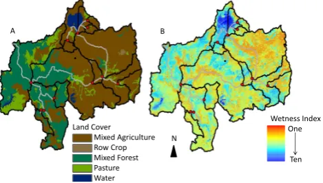
Predominant soils are generally characterized as vertisols, luvisols, and leptosols (FAO-AGL, 2003). Soil profiles in the highlands are characterized by permeable soils, under-lain by bedrock at depth. Soils are generally deeper in the lower reaches of the basin while soil depth is less on the steeper slopes. The basin is predominantly agricultural in the Highland portion, consisting of pasture and crops (64%) and forested (34%) in the western regions where elevations decline and slopes are steep. Water and wetland comprise (2%), (Fig. 2). Impervious surfaces or urban areas occupy <1% of the watershed and were thus excluded from consid-eration in the model.
Reach Subbasin Outlet Watershed Boundary Meteorological Station
Ribb North Marawi
Gumera
Kessie Jemma Angar
Border (El Diem)
SourceDEM
Value High : 4261 Low : 477 Elevation
4261 m 477m
0 50100 200 300 400 km
N
0 400 km
[image:4.595.311.545.66.207.2]Anjeni
Fig. 1. Digital Elevation Model (DEM), reaches, subbasins and sub-basin outlets initialized in the Blue Nile Basin SWAT model. Also displayed is the distribution of meteorological station used in the model.
AGRL AGRR FRST PAST WATR
Land Cover Mixed Agriculture Row Crop Mixed Forest Pasture Water
Wetness Index One
Ten N
A B
Fig. 2. Landuse/landcover (A) in the Blue Nile Basin (source EN-TRO), and the Wetness Index (B) used in the SWAT-WB Blue Nile Model.
The specific subbasins that were utilized were Anjeni, Gumera, Ribb, North Marawi, Angar, Jemma, Kessie, and the Ethiopian Abbay Blue Nile Basin (BNB) at El Diem. A short description of each follows.
The Anjeni watershed covers an area of 113.4 ha. The wa-tershed is oriented North-South and flanked on three sides by plateau ridges. It is located at 37◦310E and 10◦400N and lies 370 km NW of Addis Ababa to the south of the Choke Moun-tains. The mean annual rainfall is 1690 mm with a low vari-ability of 10% with mean daily temperature ranges from 9◦C to 23◦C. Agriculture is the dominant landuse. See SCRP (2000) for additional data on the Anjeni watershed.
The Gumera, Ribb, and North Marawi watersheds are lo-cated in the Lake Tana Basin, Ethiopia and range in size from approximately 1200 to 1600 km2. All are heavily (∼95%) cultivated, with elevations ranging from 1700 to 4000 m above sea level and predominant soils are generally charac-terized as chromic and haplic luvisols (FAO-AGL, 2003).
[image:4.595.311.546.279.412.2]rainfall (less than 1000 mm y−1). Agriculture dominates the landuse (90%), and elevations range from 1300 to 3800 m. Dominate soil types are eutric vertisols and eutric leptosols.
The Angar subbasin is located in the southern region of the BNB. Elevations range from 860 to 3210 m. The area has some of the highest rainfall in the entire basin (between 1200 and 2000 mm). Unlike other subbasins, Angar is pre-dominately forested, with some pastoral land (Fig. 2). The dominant soils in the basin are alisols, acrisols, nitosols and leptosols.
Kessie (Fig. 1) drains an area of approximately 65,000 km2, and integrates the Gumera, Ribb, North Marawi, and Jemma subbasin. The Kessie station is located on the main stem of the Blue Nile. Landuse above Kessie is pre-dominately agriculture, and elevations range from 1000 to nearly 4300 m.
2.4 Input data
Spatial Data: Required landscape data includes tabular and spatial soil data, tabular and spatial land use information, and elevation data. The spatial extent of upper Blue Nile Basin soils were taken from the FAO soil data base (FAO-AGL, 2003) (Fig. 2). Soil properties used in the SWAT model were obtained from several sources. Several soil properties are imbedded in the FAO soils data base, however, many proper-ties needed by SWAT are not included in the FAO soil, thus a review studies in the region, and literature search for spe-cific soil type properties was conducted. Arithmetic means were used for all soils properties for which a range of val-ues were found. We created a soil topographic index, (λ) – soil hybrid map for each subbasin and used it in place of the standard soils input map (as per Easton et al., 2008). The associated soils properties for theλ-soils hybrid map were extracted from the FAO database and look up tables were linked to the map using the ARCSWAT 9.2 interface. We lumped the watershed’sλinto 10 equal area intervals rang-ing from 1 to 10, with index class 1 coverrang-ing the 10% of the watershed area with the lowest λ (i.e. lowest propen-sity to saturate) and index class 10 containing the 10% of the watershed with the highestλ(i.e. highest propensity to saturate) (Fig. 2). These wetness index classes were inter-sected with the land use to create 962 HRUs in 16 subbasins (Fig. 2). A digital elevation model (DEM) of the basin was obtained from the International Water Management Institute (IWMI) with 76 m×76 m horizontal and 1 m vertical resolu-tions. Land use/land cover maps containing 19 land cover classifications were obtained from the Eastern Nile Techni-cal Regional Office (ENTRO), and reclassified into five dom-inant land use/land covers (Fig. 2).
2.4.1 Required meteorological data
Daily precipitation and minimum and maximum tempera-ture data were obtained from the Ethiopian Ministry of
Wa-ter Resources for 37 stations distributed throughout the basin (Fig. 1). Daily solar radiation, wind speed and humidity data were obtained from the United States National Climatic Data Center. Daily potential evapotranspiration rates were calcu-lated in the SWAT model using the Penmen-Monteith method and default values were used for all unavailable parameters.
3 Model calibration
3.1 Hydrology
The water balance methodology requires very little direct calibration, as most parameters can be determined a priori. Soil storage was calculated as the product of soil porosity and soil depth from the soils data. Soil storage values were distributed via theλdescribed above, and the effective depth coefficient (ρi, varies from 0 to 1) was adjusted along a
gra-dient inλvalues. We assume that the distribution ofρivalues
is inversely proportional toλi(averaged across each wetness
index class or HRU) and that the lowestλ,(λo) corresponds
to the highestρi(ρo) (Easton et al., 2010):
ρi=
λo
λi
(ρo). (4)
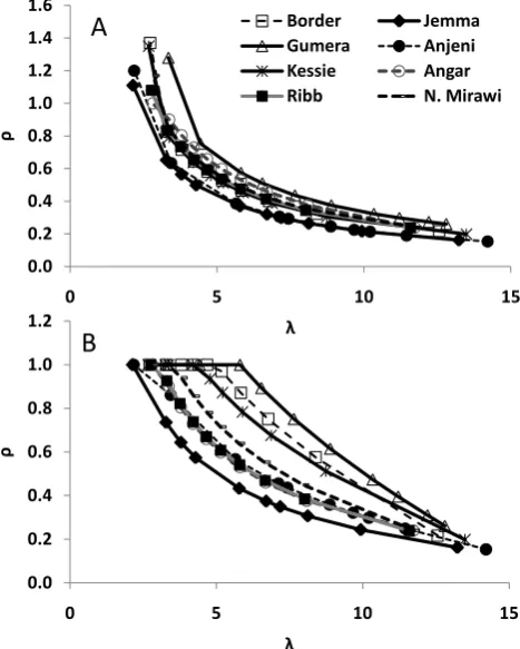
In this manner, theρi distribution (Fig. 3) requires
infor-mation on the topography (and perhaps soil) and the upper bound effective depth coefficient,ρo, for the driest wetness
index class; without any additional information about the wa-tershed, we assumeρo=1. Equation (4) gives us an initial
estimate of the distribution ofρi-values with no calibration
(Fig. 3a).
To constrain or “calibrate”ρo, we recognize that, since the
ρ-value controls how much precipitation is routed as runoff, it also controls how much precipitation water can enter the soil for a given wetness index class. Thus, a larger fraction of the precipitation that falls on an area with a largeρi will
potentially recharge the ground water than in an area with a smallρi. As a first approximation, then, we assumeρi can
be equated the ratio of groundwater recharge,qB,ito total
ex-cess precipitation.,qE,i, i.e., precipitation falling on wetness
classithat eventually reaches the watershed outlet: ρi=
qB,i
qE,i
(5) Here we assume that the area-weighted sum of ρi must
equal the watershed baseflow index,5B:
5B=
QB
QE
(6) whereQE, (mm) andQB, (mm) are the basin average excess
0.0 0.2 0.4 0.6 0.8 1.0 1.2 1.4 1.6
0 5 10 15
ρ
λ
Border Jemma
Gumera Anjeni
Kessie Angar
Ribb N. Mirawi
0.0 0.2 0.4 0.6 0.8 1.0 1.2
0 5 10 15
ρ
λ
A
[image:6.595.49.283.65.357.2]B
Fig. 3. Distribution of the effective depth coefficient (ρi) values defined by Eq. (4) (a) and Eq. (8) (b) for the various sub-basins.
The ρo-parameter (Eq. 4) can be constrained by the
area-weighted average ofρi, using Eq. 4 asρiand rearranging to
solve forρo:
ρo=
5B6Ai
6λo
λiAi
(7)
whereAi is the area of the wetness index class. Ifρo>1,
we setρo=1 and adjust the distribution ofρi iteratively until
the sum of the spatially averagedρi equal5B. To do this we
assume that for all wetness classes withλ> λ∗,ρi=1 and
belowλ∗the adjustedρi linearly approach the initial
distri-bution such that the adjusted and initialρi values are equal
at the maximumλ λM,(Fig. 1). Letρe∗be the value of the
unadjustedρi atλ∗and the adjustedρi are calculated as:
ρi= (
1 forλ0< λ < λ∗
1−ρ∗
e
λ∗−λ
M
(λiλM)+ρei forλ∗< λ < λM
(8)
While Eq. (8) can be solved iteratively by adjustingλ∗, we found the following approximation forλ∗worked well.
λ∗=λei+(λei−λ0) (9)
where λei is the value of λ where the unadjusted ρi =1
(Fig. 3) (See Easton et al., 2010 for complete details).
The primary difference between the CN based SWAT and the water balance based SWAT is that runoff is explicitly at-tributable to source areas according to a wetness index distri-bution, rather than by land use and soil infiltration properties as in original SWAT (Easton et al., 2008). Soil properties that control saturation-excess runoff generation (saturated con-ductivity, soil depth) affect runoff distribution in SWAT-WB since they are included in the wetness index via Eq. (4). Flow calibration was validated against an independent time series that consisted of at least one half of the observed data. To in-sure good calibration, we also made in-sure that our result max-imized the coefficient of determination (r2) and the Nash-Suttcliffe efficiency (NSE) (Nash and Nash-Suttcliffe, 1970). Ta-ble 1 summarizes the calibratedρi values for each wetness
index class and Table 2 summarizes the calibration statistics. Since flow data at some of the available gauge locations was available at the monthly time step (Angar, Kessie, Jemma), and daily at others (Anjeni, Gumera, Ribb, North Marawi, El Diem), the model was run for both time steps, and the results presented accordingly.
3.2 Sediment
Sediment export from the Blue Nile Basin was calibrated to measured daily sediment discharge at the El Diem station on the Sudan/Ethiopia border during 2003 and 2004 (Ahmed, 2003), and in the Anjeni micro-watershed in 1995–1996 and 2000. Since limited calibration data precludes the use of more traditional calibration and validation data sets sediment parameters were calibrated using a leave-one-out cross vali-dation time series (McCuen, 2005) to ensure the model sta-bility. For the leave-one-out cross validation one observation point is successively omitted in a series of steps. The model is calibrated with one data point withheld and the resultant calibration, based on n-1 data points, is used to predict the withheld point. This process is repeated until each data point has successively been withheld from the calibration and pre-dicted using the corresponding n-1 calibrated model. The predicted data points are then combined into a leave-one-out cross validation time series that can be compared to the data to derive goodness of fit statistics, referred to as a leave-one-out cross validation statistics. Since each point in the leave-one-out cross validation time series is predicted by a model that was calibrated with the corresponding data point excluded, it represents a model prediction that is independent of the model calibration. A small amount of sediment data was available during 1995–1996 in the Ribb subbasin, which was used as a check of the calibration.
Table 1. Effective depth coefficients (ρi) for each wetness index class and watershed in the Blue Nile Basin model from Eq. (8). The5Bis determined from baseflow separated runoff of the streamflow hydrograph and distributed.
Wetness Index Class ρi(Border) ρi(Kessie) ρi(Jemma) ρi(Angar) ρi(Gumera) ρi(Ribb) ρi(N. Marawi) ρi(Anjeni)
10 (Most Saturated) 0.22 0.20 0.16 0.15 0.26 0.24 0.24 0.15
9 0.58 0.51 0.24 0.22 0.31 0.41 0.43 0.25
8 0.75 0.68 0.31 0.26 0.40 0.51 0.53 0.30
7 0.87 0.78 0.35 0.30 0.47 0.59 0.62 0.32
6 0.97 0.87 0.37 0.34 0.61 0.66 0.69 0.36
5 1.00 0.94 0.43 0.38 0.75 0.72 0.75 0.44
4 1.00 1.00 0.57 0.42 0.89 0.80 0.83 0.46
3 1.00 1.00 0.64 0.47 1.00 0.88 0.91 0.57
2 1.00 1.00 0.74 0.52 1.00 0.99 1.00 0.86
1 (Least saturated) 1.00 1.00 1.00 0.63 1.00 1.00 1.00 1.00
*5B 0.84 0.80 0.48 0.37 0.67 0.68 0.70 0.47
∗5
Bpartitions moisture in above saturation to runoff and infiltration.
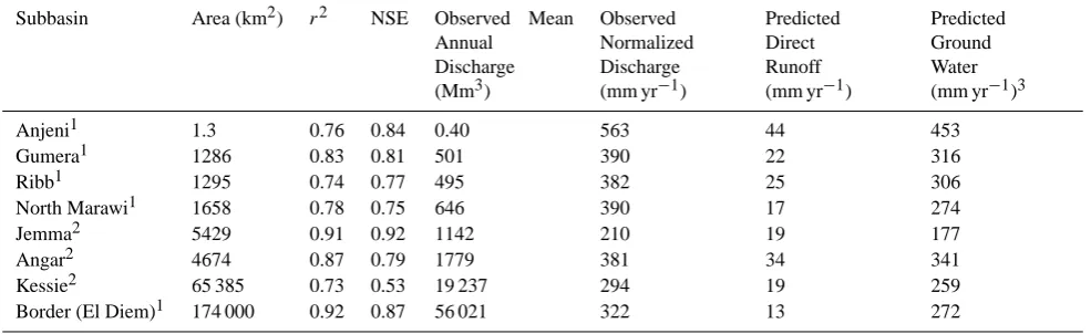
Table 2. Calibrated subbasins (Fig. 1), drainage area, model fit statistics (coefficient of determination,r2and Nash-Sutcliffe Efficiency, NSE), and observed and predicted flows.
Subbasin Area (km2) r2 NSE Observed Mean Annual
Discharge (Mm3)
Observed Normalized Discharge (mm yr−1)
Predicted Direct Runoff (mm yr−1)
Predicted Ground Water (mm yr−1)3
Anjeni1 1.3 0.76 0.84 0.40 563 44 453
Gumera1 1286 0.83 0.81 501 390 22 316
Ribb1 1295 0.74 0.77 495 382 25 306
North Marawi1 1658 0.78 0.75 646 390 17 274
Jemma2 5429 0.91 0.92 1142 210 19 177
Angar2 4674 0.87 0.79 1779 381 34 341
Kessie2 65 385 0.73 0.53 19 237 294 19 259
Border (El Diem)1 174 000 0.92 0.87 56 021 322 13 272
1Statistics are calculated on daily time step 2Statistics are calculated on monthly time step 3Includes both base and interflow.
SCRP watershed and Engda (2009) working the Andit Tid SCRP watershed showed that steeper slopes resulted in less runoff and lower erosion rates thus, we adjusted the overland Mannings-n (OV N) values as a function of slope steepness. Since SWAT is incapable of realistically modeling gully ero-sion, and gully formation can be an important erosion mech-anism in the Ethiopian highlands the soil erodibility fac-tor (USLE K) in the Modified Universal Soil Loss Equa-tion (MUSLE) (Williams, 1975) equaEqua-tion was increased by 25% to reflect this. This might result in specific field based erosion estimates being over-predict to correctly predict sub-basin scale erosion. Landscape erosion in SWAT is computed using the MUSLE, which determines sediment yield using a runoff factor that estimates the energy that governs the trans-port of eroded sediment in surface flow. Thus the sediment
delivery ratio is incorporated into the equation and does not need to be specified separately.
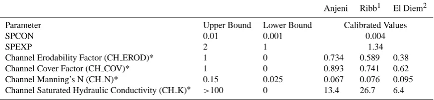
[image:7.595.51.544.317.468.2]Table 3. Parameters affecting channel degradation and deposition of sediment calibrated using leave one out cross validation for Anjeni, Ribb, and El Diem.
Anjeni Ribb1 El Diem2
Parameter Upper Bound Lower Bound Calibrated Values
SPCON 0.01 0.001 0.004
SPEXP 2 1 1.34
Channel Erodability Factor (CH EROD)* 1 0 0.734 0.589 0.38
Channel Cover Factor (CH COV)* 1 0 0.893 0.741 0.62
Channel Manning’s N (CH N)* 0.15 0.025 0.067 0.076 0.095 Channel Saturated Hydraulic Conductivity (CH K)∗ >100 0 13.4 26.7 6.4
∗Varies by reach
1Parameters calibrated for the Ribb subbbasin were transferred to Gumera, North Marawi, and the remaining land area in the Lake Tana Basin. 2Parameters calibrated at the El Diem station were transferred to all subbasins upstream except for Anjeni, and those in the Lake Tana Basin.
the respective amounts of landscape and channel sediment by comparing the sediment yield from each HRU summed within a subbasin to the channel sediment yield, which, when summed, equal the subbasin sediment export. The HRU sed-iment yield is an estimate of sedsed-iment delivery from an HRU into the main channel during the time step, while the channel sediment yield is any sediment eroded or re-entrained from the channel. Thus, sediment export from a subbasin includes both the sediment yield from the HRUs and any sediment eroded or entrained from the channel.
4 Results
4.1 Hydrology
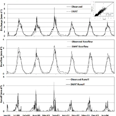
Runoff and subsurface flow from the watershed were summed at the watershed outlet to predict streamflow. The graphical comparison of the modeled and measured daily streamflow at the El Diem station at the Sudan border (e.g., integrates all subbasins above) is shown in Fig. 4. The model was able to capture the dynamics of the basin response well (NSE=0.87, r2=0.92) (Table 2, Fig. 4). Both baseflow and storm flow were correctly predicted with a slight over prediction of peak flows and a slight under prediction of low flows (Table 2), however, all statistical evaluation cri-terion indicted the model predicted well. In fact all cali-brated subbasins predicted streamflow at the outlet reason-ably well (e.g. Table 2). Model predictions showed good accuracy (NSE ranged from 0.53–0.92) with measured data across all sites except Kessie, where the water budget could not be closed; however, the timing of flow was well captured. The error at Kessie appears to be due to under estimated pre-cipitation at the nearby gauges, as measured flow was nearly 15% higher than precipitation-evapotranspiration. Never the less, the prediction is within 25% of the measured data. Ob-served normalized discharge (Table 2) across the subbasins shows a large gradient, from 210 mm at Jemma to 563 mm
at Anjeni. For the basin as a whole, approximately 25% of precipitation exits the BNB at El Diem.
Table 1 shows the adjustedρiparameter values (e.g. Eq. 8)
for the various subbasin in the BNB, and that the parameter values are scalable, and can be determined from topograph-ical information (i.e., theρi values in vary by subbasin, but
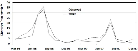
the distribution is similar, Fig. 3). The SWAT-WB model was able to accurately reproduce the various watershed re-sponses across the range of scales. Notice for instance that the hydrographs at the Border (174 000 km2) (Fig. 4), Jemma (5400 km2) (Fig. 5), Gumera (1200 km2) (Fig. 6), and An-jeni, (1.13 km2) (Fig. 7), reasonably capture the observed dy-namics (i.e., both the rising and receding limbs and the peak flows are well represented). There was a slight tendency for the model to bottom out during baseflow, likely due to over estimated ET, but the error is relatively minor. More impor-tantly the model captures peak flows, which are critical to correctly predict to asses sediment transport and erosion.
Fig. 4. Daily observed and predicted discharge, runoff, and baseflow at the Sudan border.
model reliably predicts, which is important when considering the impacts of intervention measures to augment flow.
Runoff losses predicted by the model varied across the basin as well, and were generally well corroborated by runoff estimates from baseflow separation of the streamflow hydro-graph. Predicted runoff losses (averaged across the entire subbasin) varied from as low as 13 mm y−1for the BNB as a whole subbasin to as high as 44 mm y−1 in Anjeni. Of course, small areas of the individual subbasins produce sig-nificantly higher runoff losses and others sigsig-nificantly less. These differences are well reflected in the average baseflow coefficient (5B) for the subbasins (Table 1). Notice that the
5B for Anjeni (smallest watershed, highest runoff losses) is
significantly lower than for Gumera and the Border (Table 1). A lower5Breflects less average available storage in the
wa-tershed, (i.e. more rainfall ends up as runoff). This5Bvalue
is determined from the baseflow separation of the stream-flow hydrograph (Hewlett and Hibbert, 1967), and can thus be considered a measured parameter. It is also interesting to note how the distribution of the individualρidiffers between
basins. For instance there are more classes (areas) in Anjeni and Angar that are prone to saturate, and would thus have a comparatively lower available storage than the other sub-basins. This is relatively clear in looking at the streamflow hydrographs (Figs. 4–7) where the smaller watersheds tend to generate substantially more surface runoff. Conversely, as basin size increases (Kessie, Border) the saturated frac-tion of the watershed decreases, more of the rainfall infil-trates, resulting in greater baseflow, as reflected in the higher 5B, or in terms of runoff the smaller upland watersheds have
higher runoff losses than the larger basins. This is not unex-pected, as the magnitude of the subsurface flow paths have been shown to increase with the size of the watershed, be-cause as watershed size increases more and more deep flow paths become activated in transport (Steenhuis et al., 2009).
Fig. 5. Monthly observed and predicted discharge at the Jemma subbasin.
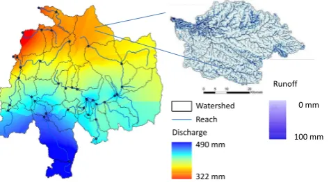
distribution of average runoff losses for the Gumera water-shed for an October 1997 event. As is evident from Fig. 8, runoff losses vary quite dramatically across the landscape, some HRUs are expected to produce no runoff, while oth-ers produced more than 90 mm of runoff. When averaged spatially at the outlet, runoff losses were 22 mm (Table 2). Other subbasins responded in a similar manner. These re-sults are consistent with data collected in the Anjeni SCRP watershed (SCRP, 2000; Ashagre, 2009), which showed that runoff losses roughly correlate with topography.
4.2 Sediment
Based on SCRP data from several of the micro watershed sites (Anjeni, Andit Tid) that shows sediment losses to be in-versely related to slope position (e.g., steeper slopes produce less erosion) it appears that the hydrologic underpinning of the SWAT-WB model (e.g. less runoff is generated on steeper slopes) provides a conceptually correct platform to asses ero-sive processes. Figure 9 shows the SWAT model predicted and observed sediment export at El Diem. The daily NSE for the simulation period was 0.74, indicating acceptable model performance. Nearly 128 million tons per year were deliv-ered during the 2 years of measurements (Ahmed, 2003), with a measured daily average during the rainy season of 1.22 million tons. The model predicted 121 million tons over the 2 yrs, with a rainy season daily average of 1.16 mil-lion tons. The average sediment concentration at El Diem was 3.751 g L−1, while the model predicted a slightly higher concentration of 4.123 g L−1. The higher concentration was somewhat counter balanced by the slightly under predicted flow (Fig. 4). Despite this, model performance appears to be adequate.
Interestingly the model predicted that landscape based ero-sion from agricultural areas, particularly tilled fields dom-inated sediment delivery to the reaches during the early part of the growing season (approximately mid-end August), after which landscape based erosion was predicted to de-crease. The reduction in landscape borne sediment reflects the growth stage of plants in the highlands, which in mid-late August are reasonably mature, or at least have devel-oped a canopy and root system that effectively reduces rill and sheet erosion (Zegeye, 2009). After that sediment export
from the various subbasins was controlled by channel erosion and re-entrainment/re-suspension of landscape sediment de-posited in the reaches in the early part of the growing season. This sediment was subsequently mobilized during the higher flows that typically peak after the sediment peak is observed [e.g., the sediment peak occurs approximately two weeks (in July) before the flow peak (in August)] (compare Figs. 4 and 9). Figure 10 shows significant hysteresis between the rising and receding limbs of the sediment concentration hydrograph (natural log transformed data). The sediment concentration on the rising limb of the hydrograph has a lower slope, and higher intercept than the receding limb. While we do not know the mechanisms behind this difference it seems logi-cal that there are different processes controlling the sediment dynamics during different parts of the year (e.g., as illus-trated by the hysteresis). This, of course, has implications for reservoir management in downstream countries, in that much of the high sediment flow can pass through the reser-voir during the rising limb, and the relatively cleaner flows stored during the receding limb. Never the less, the sheer volume of sediment exported from the Ethiopian highlands threatens many downstream structures regardless of their op-eration and clearly impacts agricultural productivity in the highlands.
SWAT predicts that the sediment later in the growing sea-son is channel based (either from landscape sources de-posited during lower velocity flows or directly from the chan-nel itself), However, there is significant gully erosion in many areas of the highlands, that, in fact become active at approx-imately the same time as the flow peak occurs and SWAT predicts channel processes to be the source. Gully activa-tion occurs once the soil has wet up and lost its cohesive na-ture. Soil wets up from the interflow from upslope areas, and thus it does not always occur simultaneously with landscape sources of erosion (Tebebu, 2009; Zegeye, 2009). In actual-ity, the receding limb of the sediment hydrograph (Fig. 10) is likely a combination of both channel re-suspension of land-scape sources, channel erosion, and gully erosion. However, it should be noted that much of the main stem of the Blue Nile cuts through a rocked canyon composed of basalt lavas, granites, and sandstones, and thus direct channel and bank erosion is likely a small contributor. Smaller reaches where flow velocities are high likely do contribute sediment from both channel and bank sources.
Fig. 6. Daily observed and predicted discharge from the Gumera subbasin.
Fig. 7. Daily observed and predicted discharge from the Anjeni micro watershed.
Watershed
Reach
GW(mm) 477
187
Watershed Reach
490 mm
322 mm Discharge
Gumera _STI
Value
High : 11.6494
Low : 2.93952 0 mm
100 mm Runoff
Fig. 8. Predicted average yearly spatial distribution of discharge in the Blue Nile Basin (main) and predicted runoff distribution in the Gumera sub watershed for an October 1997 event (inset).
shows the measured and predicted sediment export for the Border, Ribb and Anjeni. While the total sediment export in-tuitively increases with basin size, the normalized sediment export (t km2) was inversely proportional to the basin size (Table 4). This is a direct result of the difference in the base-flow coefficients (5B) among the various sized basins, (e.g.,
0.47 for Anjeni to 0.84 for the Border).
[image:11.595.51.288.428.559.2]Table 4. Model fit statistics (coefficient of determination,r2and Nash-Sutcliffe Efficiency, NSE), and sediment export for the Anjeni, Ribb, and Border (El Diem) Subbasins during the rainy season.
Subbasin r2 NSE Measured Sediment Export Modeled Sediment Export Modeled Sediment Export
ton d−1 ton km2d−1
Anjeni 0.80 0.74 239 227 201.2
Ribb∗ 0.74 0.71 30,657 29 456 22.7
Border (El Diem) 0.67 0.64 1 229 821 1 232 468 7.1
∗Consists of four measurements.
Table 5. Annual predicted sediment yield for each wetness index class (basin average) and for the pasture, crop, and forest land covers. Wetness Index one produces the lowest runoff; wetness class ten produces the most runoff.
Landcover Wetness Index Class Sediment Yield (ton ha yr−1)
One Two Three Four Five Six Seven Eight Nine Ten Pasture 1.2 3.6 3.4 3.6 3.9 5.6 8.8 10.1 12.5 14.3 Crop 2.1 2.3 3.4 3.5 4.6 5.9 10.7 9.9 14.2 15.6 Forest 0.3 0.5 0.9 1.5 1.7 1.6 2.8 3.1 3.7 4.1
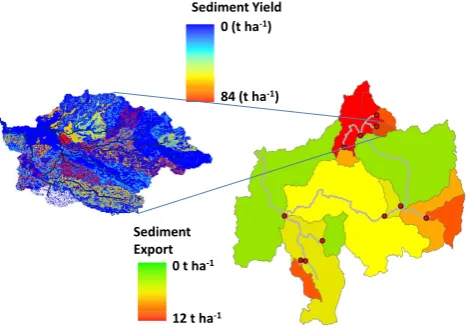
runoff levels in the basin. The Fincha region, in the south-ern area of the basin, was not specifically a subbasin in the model, but the area was also predicted to have high sediment yields. Conversely, sediment yields are considerably lower (on average) in subbasins along the along the main stem of the Blue Nile (Fig. 12), mainly a result of the lower slopes, and more forested areas, particularly in the north-western re-gion. However, the model still predicts some large sources of sediment in these areas, specifically, agricultural land on steep, or saturated soils.
The predicted gradient in sediment yield within subbasins is illustrated in Fig. 12. Inset, where the Gumera watershed in the Lake Tana subbasin is shown. The model predicts only a relatively small portion of the watershed to contribute the bulk of the sediment (75% of the sediment yield originates from 10% of the area, while much of the area contributes low sediment yield. The high sediment yield areas are gen-erally predicted to occur at the bottom of steep agricultural slopes, where subsurface flow accumulates, and the stability of the slope is reduced from tillage and or excessive livestock traffic. Note also that these are the areas that gully formation is likely (Tebebu, 2009; Tebebu et al., 2010).
5 Discussion
Flows in the Blue Nile Basin in Ethiopia show large variabil-ity across scales and locations. Sediment and water yields from areas of the basin range more than an order of mag-nitude. Smaller basins showed both higher runoff and sedi-ment losses per unit area. Furthermore, even within smaller watersheds such as the Anjeni micro-catchment there are
ar-eas that produce virtually no runoff or erosion, and arar-eas that produce very high levels of both runoff and erosion. Much of the erosion in the Anjeni catchment was generated from a large gully in the low-lying area (Ashagre, 2009). While the SWAT model cannot predict the formation of gullies, the SWAT-WB model can indicate where the formation of gul-lies is probable. In most cases gulgul-lies form where the soil is saturated either from a large contributing area for water to accumulate or where slopes flatten and the effective hy-draulic conductivity is reduced (Tebebu et al., 2010). These areas tend to occur at the bottom of long slopes in the wetter valley bottom areas, which, not surprisingly also support in-tensive animal agriculture. Indeed, Table 5 shows these areas (higher wetness index classes, or areas with higherλvalues) to produce substantially higher sediment yields than other ar-eas, inevitable, since these areas produce higher runoff losses as well. This seems to agree with what has been observed in the basin (e.g., Tebebu, 2009), and points towards the need to develop management strategies that incorporate landscape position into the decision making process. Interestingly, both pasture and crop land in the higher wetness classes had ap-proximately equivalent sediment losses, while forest in these same areas had substantially lower erosive losses, likely due to the more consistent ground cover and better root system.
[image:12.595.127.469.241.308.2]0 30000 60000 90000 120000 150000 180000
Jun-03 Sep-03 Dec-03Mar-04 Jun-04 Sep-04
Cu
m
lativ
e
Sed
im
e
n
t
Yei
ld
/E
xp
o
rt
(1000
to
n
s)
Landscape Sediment
[image:13.595.115.484.64.151.2]Channel Sediment
[image:13.595.67.269.211.340.2]Fig. 9. Observed and SWAT modeled sediment export at the Sudan/Ethiopia border (a) and the predicted landscape sediment yield and channel sediment export (b).
Fig. 10. Natural log of the sediment concentration vs natural log of the flow at El Diem gauge for the rising and receding limb of the discharge hydrograph.
large scale watershed models are crude, at best, and do not incorporate the appropriate mechanistic processes to reliably predict when and where erosion occurs, at least at the scale needed to manage complex landscapes. For instance, the MULSE routine in SWAT does not predict gully erosion, which is a large component of the sediment budget in the Blue Nile. To correctly capture the integrated watershed wide export of sediment the original SWAT predicts ero-sion to occur more or less equally across the various land covers (e.g., crop land produces approximately equal erosive losses, pasture produces approximately equal erosive losses) provided they have similar soils and land management prac-tices throughout the basin. The modified version of SWAT used here recognizes that different areas of a basin (or land-scape) produce differing runoff losses and thus differing sed-iment losses (Table 5). However, all crop or pasture with in a wetness index class in the modified SWAT produces the same erosive losses, and is rill or sheet erosion (as predict by MUSLE), not gully erosion. Thus, rill and sheet erosion are likely over predicted to obtain the correct sediment export from the basin.
It is interesting to note that the model can predict that the sediment load peaks before the flow, and that it predicts the cause to be the result of relating the sediment concentration to the time when the watershed becomes covered by vege-tation. The model indicates that later in the rainy season on
the receding limb of the sediment hydrograph, sediment ex-port is dominated by channel processes. However, as noted earlier, gully erosion is also a large sediment source later in the season, as interflow causes the soil to saturate and in-creases the hydrostatic pressure in the gully (e.g., a water table forms above the gully bottom) (Tebebu et al., 2010). Based on watershed outflow measurements, we cannot dis-criminate between these mechanisms since both signals ap-pear at the same time. However, the gully explanation seems to be reasonable since during the rainy season high sedi-ment concentrations are observed in the basin and relatively sediment free water is observed after the surface runoff has ended, and interflow continues.
The next logical work with these basin scale models should explore incorporating more realistic processes con-trolling erosion. Models such as the Water Erosion Predic-tion Project (WEPP) model incorporate mechanistic process based erosion modeling capabilities, but are applicable only to the hillslope or small watershed scale. There is an addi-tional need to increase the parsimony of the basin scale mod-els. The modification made to SWAT (SWAT-WB) provides a good first step towards more correctly capturing distributed hydrologic responses while significantly reducing calibration needs. This provides a useful platform on which to base sed-iment predictions, but still does not overcome the inherent weakness of empirical erosion routines such as those used in SWAT. Models that utilize USLE and its derivates often re-quire (excessive) calibration, and there exist very few data sets that can reliably provide both the integrated and dis-tributed data to calibrate against. Translating these capabil-ities to basin scale models will be challenging, but are crit-ical to the future of land and water resource management, particularly in regions where there is little measured data to calibrate these models to.
6 Conclusions
Fig. 11. Measured and SWAT predicted sediment export from the Anjeni micro-watershed.
Combine_Wate2
High : 65535
Low : 0
Sediment Yield 0 (t ha-1)
84 (t ha-1)
SourceDEM
Value
High : 4261
Low : 477
0 t ha-1
12 t ha-1
Sediment Export
Fig. 12. Sediment export (t ha−1yr−1) in the subbasins predicted by the model (main figure) and sediment yield by hydrologic re-sponse unit (HRU) for the Gumera subbasins (inset).
initialize the model to predict runoff are obtained from base-flow separation of the hydrograph (5B), and from
topo-graphical information derived from a DEM and soils data (λ). The reduced parameterization/ calibration effort is valu-able in environments such as Ethiopia where there are limited data to build and test complicated biogeochemical models.
Using the model we were able to quantify the relative con-tributions from the various areas of the BNB with relatively good accuracy, particularly at a daily time step. The anal-ysis showed that not all subbasins contribute flow or runoff equally. In fact there is large variation in average flow and runoff across the watershed. Additionally, within any one watershed the model indicates that there are areas that pro-duce significantly more runoff and areas that propro-duce almost no runoff, which, of course has implications for the manage-ment of these areas. This model is helpful to identify areas of a basin that are susceptible to erosive or other contaminant losses, due to high runoff production. These areas should be targeted for management intervention to improve water qual-ity.
An analysis of sedimentation and erosion in the Blue Nile Basin was conducted to determine the relative sources of sed-iment. The model showed good fit to observed sediment load at the El Diem station. The model predicted several areas of the watershed to be relatively large sediment contribu-tors, however, more work should be done to corroborate the subbasin and intra-watershed predicted sediment yields. The processes governing the erosion and sedimentation dynamics are not fully understood in the Blue Nile, thus the sediment predictions should be considered tentative until more testing is done.
Acknowledgements. We would like to the Amhara Regional
Agricultural Research Institute, the Ethiopian Ministry of Water Resources, and ENTRO for providing data. Funding for the work was provided in part by the CPWF-19 Upstream-Downstream Project, Cornell University, and by the US Dept. of Agriculture International Science and Education Competitive Grants Program.
Edited by: M. Gebremichael
References
Ahmed, A. A.: Sediment Transport and Watershed Management Blue Nile System. Friend/Nile Project report, UNESCO, Khar-toum, Sudan, 2003.
Arnold, J. G., Allen, P. M., Muttiah, R., and Bernhardt, G.: Au-tomated base-flow separation and recession analysis techniques, Ground Water, 33, 1010–1018, 1995.
Arnold, J. G., Srinivasan, R., Muttiah, R. S., and Williams, J. R.: Large area hydrologic modeling and assessment part I: model development, J. Am. Water Resour. Assoc. 34(1), 73–89, 1998. Ashagre, B. B.: Formulation of best management option for a
water-shed using swat (Anjeni waterwater-shed, Blue Nile Basin, Ethiopia), M.P.S Thesis. Cornell University, Ithaca, NY, USA, 2009 . Awulachew, S. B., Yilma, A. D., Luelseged, M., Loiskandl, W.,
Ayana, M., and Alamirew, T.: Water Resources and Irrigation Development in Ethiopia, Colombo, Sri Lanka: International Water Management Institute, Working paper 123, 78 pp., 2007. Bayabil, H. K.: Are runoff processes ecologically or
[image:14.595.51.285.240.404.2]the Maybar watershed, M.P.S Thesis. Cornell University, Ithaca, NY, USA, 2009.
Beven, K. J. and Kirkby, M. J.: Towards a simple physically-based variable contributing model of catchment hydrology, Hydrol. Sci. Bull. 24(1), 43–69, 1979.
Collick, A. S., Easton, Z. M., Adgo, E., Awulachew, S. B., Gete, Z., and Steenhuis, T. S.: Application of a physically-based water bal-ance model on four watersheds throughout the upper Nile basin in Ethiopia, Hydrol. Proc., 23, 3718–372, doi:10.1002/hyp.7517, 2009.
Conway, D.: A water balance model of the upper Blue Nile in Ethiopia, Hydrol. Sci., 42(2), 265–286, 1997.
Constable, M.: Resource of Rural Development in Ethiopia. Ethiopian High lands Reclamation Study, FAO/Ministry of Agri-culture, Addis Ababa, Working Paper 17, 1984.
Derib, S. D., Assefa, T., Berhanu, B., and Zeleke, G.: Impacts of micro-basin water harvesting structures in improving vegetative cover in degraded hillslope areas of north-east Ethiopia, Range-land Journal, 31, 259–265, 2009.
Easton, Z. M., D. R. Fuka, M. T. Walter, D. M. Cowan, E. M. Schneiderman, and T. S. Steenhuis (2008), Re-conceptualizing the Soil and Water Assessment Tool (SWAT) model to predict runoff from variable source areas, J. Hydrol., 348(3–4), 279–291. Easton, Z. M., Walter, M. T., Fuka, D. R., White, E. D., and Steen-huis, T. S.: A simple concept for calibrating runoff thresholds in quasi-distributed variable source area watershed models, Hydrol. Proc., submitted, 2010.
Engda, T. A.: Modeling rainfall, runoff and soil loss relationships in the Northeastern Highlands of Ethiopia, Andit Tid watershed, M.P.S Thesis, Cornell University, Ithaca, NY, USA, 2009. FAO-AGL: WRB Map of World Soil Resources. Land and Water
Development Division, Food and Agriculture Organization of the United Nations. Available at: http://www.fao.org/ag/agl/agll/ wrb/soilres.stm, last access: June 2010), 2003.
Garzanti, G., Ando, S., Vezzoli, G., Megid, A. A. A., and El Kam-mar, A.: Petrology of Nile River sands (Ethiopia and Sudan) Sed-iment budgets and erosion patterns, Earth Planet. Sci. Lett., 252, 327–341, 2006.
Gizawchew, A.: Soil erosion assessment: Approaches, magnitude of the problem and issues on policy and strategy development (Region 3), paper presented at the Workshop on Regional Natural Resources Management Potentials and Constraints, Bahir Dar, Ethiopia, 11–13 January 1995, Bureau of Natural Resources and Environmental Protection, Bahir Dar, Ethiopia, 9 pp., 1995. Grunwald, S. and Norton, L. D.: Calibration and validation of a
non-point source pollution model, Agr. Water Manag. 45, 17–39, 2000.
Guswa, A. J., Celia, M. A., and Rodriguez-Iturbe, I.: Models of soil dynamics in ecohydrology: A comparative study, Water Resour. Res., 38(9), 1166–1181, 2002.
Herweg, K. and Stillhardt, B.: The variability of soil erosion in the Highlands of Ethiopia and Eritrea. Research Report 42, Centre for development and Environment, University of Berne, Switzer-land, 1999.
Hewlett, J. D. and Hibbert, A. R.: Factors affecting the response of small watersheds to precipitation in humid area. Proceedings of International Symposium on Forest Hydrology, edited by: Sop-per, W. E. and Lull, H. W., Pergamon Press, Oxford, England, 275–290, 1967.
Hurni, H.: Land degradation, famines and resource scenarios in Ethiopia, In World Soil Erosion and Conservation, Cambridge University Press, Cambridge, 1993.
Liu, B. M., Collick, A. S., Zeleke, G., Adgo, E., Easton, Z. M., and Steenhuis, T. S.: Rainfall-discharge relationships for a mon-soonal climate in the Ethiopian highlands, Hydrol. Proc., 22(7), 1059–1067, 2008.
McCuen, R. H.: Accuracy assessment of peak discharge models, J. Hydrol. Eng., 10(1), 16–22, 2005.
MoWR (Ministry of Water Resources): Ethiopian water sector strat-egy, MoWR, Addis Ababa, 2002.
Nash, J. E. and Sutcliffe, J. V.: River flow forecasting through conceptual models. Part I a discussion of principles, J. Hydrol. 10, 282–290, 1970.
SCRP (Soil Conservation Reserve Program): Area of Anjeni, Gojam, Ethiopia: Long-term Monitoring of the Agricultural Environment 1984–1994, 2000 Soil Erosion and Conservation Database, Soil Conservation Research Programme. Centre for Development and Environment in association with the Ministry of Agriculture, Ethiopia, Berne, Switzerland, 2000.
Steenhuis, T. S., Collick, A. S., Easton, Z. M., Leggesse, E. S., Bayabil, H. K., White, E. D., Awulachew, S. B., Adgo, E., and Abdalla-Ahmed, A.: Predicting discharge and erosion for the Abay (Blue Nile) with a simple model, Hydrol. Proc., 23, 3728– 3737, 2009.
Swain, A.: Ethiopia, the Sudan, and Egypt: The Nile River dispute. The Journal of Modern African Studies. 35, 675–694, 1997. Tebebu, T. Y.: Assessment of hydrological controls on gully
for-mation near Lake Tana, northern Higlands of Ethiopia, M.P.S Thesis, Cornell University, Ithaca, NY, USA, 2009.
Tebebu, T. Y., Abiy, A. Z., Dahlke, H. E., Easton, Z. M., Zegeye, A. D., Tilahun, S. A., Collick, A. S., Kidnau, S., Moges, S., Dadgari, F., and Steenhuis, T. S.: Surface and subsurface flow effect on permanent gully formation and upland erosion near Lake Tana in the Northern Highlands of Ethiopia, Hydrol. Earth Syst. Sci. Discuss., 7, 5235–5265, doi:10.5194/hessd-7-5235-2010, 2010. Werner C.. Soil Conservation Experiment in the Anjeni Area,
Go-jam Research Unit (Ethiopia). University of Berne, Switzerland, Soil Conservation Research Project 13, 1986.
White, E. D., Easton, Z. M., Fuka, D. R., Collick, A. S., Adgo, E., McCartney, M., Awulachew, S. B., Selassie, Y., and Steen-huis, T. S.: Development and application of a physically based landscape water balance in the SWAT model, Hydrol. Proc., doi:10.1002/hyp.7876, 2010.
Williams, J. R.: Sediment-yield prediction with universal equation using runoff energy factor, In Present and Prospective Technol-ogy for Predicting Sediment Yield and Sources: Proceedings of the Sediment Yield Workshop, USDA Sedimentation Lab., Ox-ford, MS, 28–30 November, ARS-S-40, 1972, 1975.