Sediment transport modelling in a distributed physically based hydrological catchment model

www.hydrol-earth-syst-sci.net/15/2821/2011/ doi:10.5194/hess-15-2821-2011

© Author(s) 2011. CC Attribution 3.0 License.

Earth System

Sciences

Sediment transport modelling in a distributed physically based

hydrological catchment model

M. Konz1, M. Chiari2, S. Rimkus1, J. M. Turowski3, P. Molnar1, D. Rickenmann3, and P. Burlando1

1_{Institute of Environmental Engineering, ETH Zurich, Wolfgang-Pauli-Str. 15, 8093 Zurich, Switzerland} 2_{Institute of Mountain Risk Engineering, University of Natural Resources and Life Sciences, Peter Jordanstr. 82,}

1190 Vienna, Austria

3_{Mountain Hydrology and Torrents, Swiss Federal Research Institute, WSL, Z¨urcherstr. 111, 8903 Birmensdorf, Switzerland}

Received: 10 August 2010 – Published in Hydrol. Earth Syst. Sci. Discuss.: 4 October 2010 Revised: 10 August 2011 – Accepted: 26 August 2011 – Published: 9 September 2011

Abstract. Bedload sediment transport and erosion processes in channels are important components of water induced natu-ral hazards in alpine environments. A raster based distributed hydrological model, TOPKAPI, has been further developed to support continuous simulations of river bed erosion and deposition processes. The hydrological model simulates all relevant components of the water cycle and non-linear reser-voir methods are applied for water fluxes in the soil, on the ground surface and in the channel. The sediment transport simulations are performed on a sub-grid level, which allows for a better discretization of the channel geometry, whereas water fluxes are calculated on the grid level in order to be CPU efficient. Several transport equations as well as the effects of an armour layer on the transport threshold dis-charge are considered. Flow resistance due to macro rough-ness is also considered. The advantage of this approach is the integrated simulation of the entire basin runoff response combined with hillslope-channel coupled erosion and trans-port simulation. The comparison with the modelling tool SETRAC demonstrates the reliability of the modelling con-cept. The devised technique is very fast and of comparable accuracy to the more specialised sediment transport model SETRAC.

Correspondence to: M. Konz et al. ([email protected])

1 Introduction

a sediment transport equation together with the so-called Exner equation to account for sediment transport and storage effects in the riverbed. Examples are the one dimensional 3ST1D model (Papanicolaou et al., 2004), the 1.5 dimen-sional FLORIS-2000 model (Reichel et al., 2000) or the semi two-dimensional stream tube SDAR model (Bahadori et al., 2006). Most two-dimensional bedload transport models have been developed for large riverine or estuarine environments. An example of a two-dimensional model applicable for steep slopes is the Flumen model (Beffa, 2005). The SETRAC model (Rickenmann et al., 2006; Chiari et al., 2010b) has specifically been developed for simulations of steep alpine torrents. These very specialized models allow for simula-tions of sediment transport in a detailed way. The drawback of these models is, however, that important feedback mech-anisms as well as the seriality of processes are hard to study due to the separate treatment of the streamflow modelling and the sediment transport. The answer to this limitation can come from integrated models, which account for both basin hydrology and processes driven by hydrological response, like soil slips and sediment transport in channels. Thus, sediment transport accounting hydrological models were de-veloped, which consider sediment transfer processes at the catchment scale, within the framework of a classical rainfall-runoff model. Examples are the ETC rainfall-rainfall-runoff-erosion model (Mathys et al., 2003), the SHESED model (Wicks and Bathurst, 1996), the DHSVM model (Doten et al., 2006) or the PROMAB- GIS model (Rinderer et al., 2009).

The rather limited complexity of some of these models is, however, not always adequate to simulate the continuous process of erosion and sediment transport in mountainous catchments. Some other models were conceived for appli-cations in basins characterised by gentle topography and do not include equations specifically suitable for steep channels, which are typical of mountain basins.

Accordingly, this paper focuses on the simulation of sedi-ment transport in steep torrents of alpine catchsedi-ments. Mod-els for simulations of mountainous catchments require spe-cific modules for simulation of hydrological processes such as snow and glacier melt and routing, while a detailed de-scription of the highly variable channel geometry is needed for the sediment transport simulations. In fact, geometrical properties like channel bed slope and channel width are im-portant variables, which control hydraulics and consequently bedload transport. Usually, a high resolution grid is a prereq-uisite for the detailed description of channel geometry. How-ever, model simulations demand more CPU with increasing resolution and basin wide simulations become inefficient and slow. In this paper we added a module for the simulation of the temporal evolution of river bed sediment dynamics at the catchment scale to the distributed physically-based hydrolog-ical model TOPKAPI. The innovative aspect of the newly in-troduced sediment module is the sub-grid simulation of the sediment routing, which takes advantage of the more detailed description of the channel geometry at the sub-grid level, and

the efficient hydrological and hydraulic simulations on the coarser grid level used for the simulation of the catchment hydrology. The aim of this paper is to describe the imple-mentation of the sub-grid sediment modelling scheme and to present the evaluation of the newly developed sediment module against the more specialized SETRAC model as a model inter-comparison. In order to corroborate the findings from the intercomparison, we use, rather than a hypothet-ical case study, the 2005 flood event in the Bernese Alps, Switzerland. Although the available data base of this event has been reconstructed from post-event observations and is thus affected by some limitations in terms of error quantifi-cation, it provides a case to test the model in a realistic basin and channel morphology and topography context. As such, it allowed, as further discussed in the subsequent sections, to highlight the relevance of using a reduced energy slope due to macro-roughness flow resistance. It must be therefore clear to the reader that the aim of this work is not to repro-duce the sediment balance of the storm event in detail, being this a difficult task due to the hardly quantifiable observa-tional error: it is rather a comparison of a model specialized in channel sediment transport with a more agile and, above all, catchment scale hydrological model capable of matching the performance of the specialized model.

2 Study site and extreme event in August 2005

Many regions in Austria, Switzerland and Germany were af-fected by the flood events in August 2005 (MeteoSchweiz, 2006). A massive cyclone over the northern part of Italy caused heavy rainfall particularly from 21–22 August 2005. The period of relevant precipitation was about four days, whereas thunderstorms were not of major importance. In Switzerland the whole north-alpine region was affected by heavy rainfall that triggered widespread flooding. The high-est precipitation sums for a 72-h period were measured in Switzerland, where more than 250 mm were observed across the Alps, with the highest sums observed in Gadmen, 320 mm, Rotschalp, 283 mm, Weesen, 277 mm, and Amden, 267 mm (MeteoSchweiz, 2006).

-6-

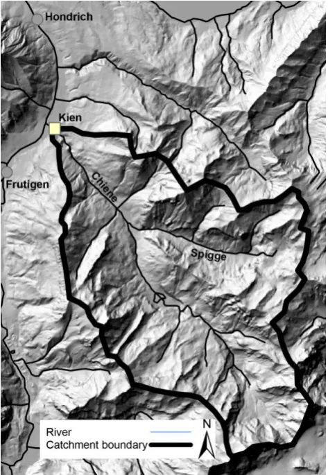
Fig. 1: Chiene catchment area and location of gauging stations for discharge reconstruction.

Fig. 1. Chiene catchment area and location of gauging stations for

discharge reconstruction.

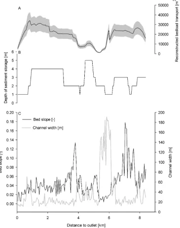
The Chiene is a steep mountain stream with a mean chan-nel gradient of 0.05. The slope is ranging from 0.004 in the flat middle reaches up to 0.17 in the steepest reaches (Fig. 2c). The channel width has a maximum of around 150 m between 5.5 and 6.2 km. The initial sediment stor-age depth was estimated in the field between 1 and 5 m. This estimate refers to a possible volume of sediment which may have been entrained during the flood from the bed and the banks, and this volume is divided by the channel width and the unit stream length of 1 m. This assessment was made for all channel reaches, and the estimated value depends for example on the presence of large boulders inhibiting or slow-ing down erosion or of bedrock limitslow-ing the maximum ero-sion depth. The grain size distributions were estimated with a transect-by-number analysis and evaluated after Fehr (1986), values were taken from Chiari et al. (2010b). Two LiDAR based digital elevation models (DEM) are available for the catchment, representing the pre- and post-flood situation. Morphologic changes in torrents and mountain rivers are only caused by major flood events. No other flood events have been reported for the time span between the two

Li-DAR flights. Chiari et al. (2010b) derived the transport vol-umes from these LiDAR based DEMs.The volumetric anal-ysis was carried out using the methodology illustrated by Scheidl et al. (2008) and compared qualitatively with aerial photographs and completed with data from sediment redis-tribution during the flood recovery phase (LLE Reichenbach, 2006). During the event, about 120 000 m3of bedload were mobilized. Most of the material was deposited in the flat mid-dle reaches (5.3 km to 6 km) and in the village of Kien, close to the confluence with Kander river. The LiDAR analysis indicated that there was more deposition in the flat middle reaches (5.5 km) than sediment input from upstream areas not covered by the LiDAR flight. Therefore, we considered at 8.3 km (see Fig. 2a) a sediment input of about 20 000 m3 from that area, which can be assumed, if we consider an error estimate comparable to that found by Scheidl et al. (2008) to be in agreement with field observations (LLE Reichenbach, 2006). This allowed assessing the sediment supply over the entire catchment area. We refrain here from a detailed dis-cussion about error estimates of the reconstructed sediment supply, since we use these data only as qualitative reference for the comparison between the two models. An error of ±25 % of the reconstructed sediment transport rates as sug-gested by Scheidl at al. (2008) is shown in Fig. 2a as grey band around the estimated value.

3 The TOPKAPI model

TOPKAPI has originally been developed at the University of Bologna (Italy) as a physically based distributed hydro-logical catchment model (Todini and Ciarapica, 2001; Liu and Todini, 2002; Liu et al., 2005). The model simulates all relevant components of the water balance and models the rainfall-runoff (R-R) processes by means of non-linear reser-voir equations, which represent drainage of the soils, over-land flow and channel flow and are obtained by the integra-tion of the topographic kinematic approximaintegra-tion of the flow equations (Todini and Ciarapica, 2001). The relevant infor-mation about river network topology, surface roughness and soil characteristics are obtainable from digital elevation mod-els, soil and land use maps.

Fig. 2. Properties of the Chiene river and observations of bedload transport. A: Reconstructed bedload transport, the grey band indicates a

±25 % error band, B: initial depth of sediment storage, C: bed slope of the river and channel width.

3.1 The R-R model components in TOPKAPI

The R-R model components can by grouped into four major modules: (i) the module to generate spatially distributed me-teorological input variables, (ii) the snow and glacier mod-ule, (iii) the soil and runoff generation modmod-ule, and (iv) the channel routing module. The R-R response is simulated in a distributed grid-based approach and within one time step the model simulates the water cycle components for each grid cell accounting for topographic constraints. Meteorological input variables (temperature and precipitation) can be

yields the soil water content. Overland flow occurs if the maximum soil water storage is exceeded. This is equivalent to a saturation excess runoff generation mechanism. Actual evapotranspiration is calculated as a function of the soil water content and potential evapotranspiration if the water content is below a certain threshold. Otherwise, actual evapotranspi-ration equals the potential evapotranspievapotranspi-ration, which is com-puted with the Makkink approach (Deyhle et al., 1996).

Water fluxes in the soil are obtained by combining the dy-namic equation (Eq. 1) with the equation for continuity of mass (Eq. 2).

q=tan(β)ksL2b (1)

p=(ϑs−ϑr)L

∂2 ∂t +

∂q

∂x (2)

Hereq is the horizontal flow in the soil in m2s−1,pis the intensity of vertical inflow in m s−1,t is time in s, x is the direction of flow along a cell in m,β is the slope angle as radiance,bis an empirical parameter which depends on the soil characteristics,ksis the saturated hydraulic conductivity

in m s−1,Lis the thickness of the soil layer in m,2is the mean value along the vertical profile of the soil water content, ϑsis the saturated soil water content andϑris the residual soil

water content.

Two soil layers can be used to simulate interflow and base flow components. Overland flow is computed with a com-parable approach but Manning’s formula is used in place of the dynamic equation. Soil erosion on hillslopes is computed based on simulated overland flow. The hillslopes are coupled to the river channel and the mobilised mass fills the sediment storage of the river if the sediment reaches the river. The hillslope erosion module is, however, not discussed here and has not been used in this study, because the focus of this pa-per is set on channel sediment transport simulations during flood events and the benchmark model SETRAC does not simulate hillslope erosion. An additional module, which has been added to the model but is not described here, allows the simulation of slope failures by computing the factor of safety on the basis of the soil water dynamics, thus allowing to compute localized sediment supply. Finally, flow routing in the channel is particularly important for sediment trans-port simulations and is therefore described in detail in the next section.

3.2 Channel flow routing

Channel flow is described with a kinematic wave approxi-mation similar to overland flow, thus describing the flow dy-namics by means of Manning’s formula (Eq. 3) and of the continuity equation shown in Eq. (4), that is

qc=

1 nc √ S _B C 2/3 By 5 /3 c (3) ∂Vc

∂t = rc+Q

u

c ₋

qc (4)

where qc is the horizontal flow in the channel in m3s−1,

nc Manning’s friction coefficient for channel roughness in

m−1/3s,Sis the bed slope,B is the channel width in m,C is the wetted perimeter,ycis the water depth in the channel

in m,Vcis the water volume in the channel in m3,t is time

in s,rcis the lateral drainage input in m3s−1, andQuc is the

inflow discharge from the channel reach of the upper cells in m3s−1. The channels are assumed to be rectangular.

The three non-linear reservoir equations representing soil flow, overland flow and channel flow can be solved analyt-ically as discussed in detail by Todini and Mazzetti (2008). This enables a very efficient computation of the flow pro-cesses.

Discharge is simulated in each grid cell that is assigned to as a channel cell. In TOPKAPI the cell length is automati-cally the length of the river section in this cell, whereas the channel width can be defined as a fraction of the cell size. The bed slope is derived from the DEM.

Flow resistance due to grain roughness plays a crucial role in steep headwater streams and is considered in TOPKAPI by a variable Manning friction coefficient. The Manning coef-ficient conventionally used by TOPKAPI has been modified to account for dependence on flow depth, and is therefore expressed as a function of discharge, bed slope and the char-acteristic grain size of the channel bed material that is

forS≥0.008 (5)

and nc=

S0.03d₉₀0.23 4.36g0.49_q0.02

c

forS≤0.008 (6)

wheregis the gravity acceleration andd90is the grain size

of the bed material for which 90 % of the bed material is finer by weight. These equations were derived from more than 300 field measurements in torrents and gravel bed rivers (Rickenmann, 1994, 1996).

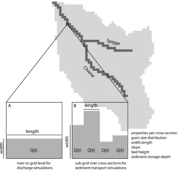
3.3 Sediment transport in TOPKAPI 3.3.1 The sub-grid modelling scheme

Fig. 3. Sub-grid concept of river cross-sections. A: River representation for hydraulic simulations on the grid level; B: Sub-grid cross-sections

for sediment transport simulations.

Fig. 3b). There is no feedback mechanism between sedi-ment transport simulations and hydraulic simulations, which means that for the hydraulic simulations the channel geome-try is constant through time.

In order to avoid rapid exhaustion of the sediment stor-ages the time step length can be decreased to a fraction of the global time step used for the hydrological simulations. The choice of the sub-grid time step is further discussed in Sect. 6. The sediment transport simulations described in the following sections are conducted on the sub-grid level.

3.3.2 Sediment transport capacity

For the calculation of the sediment transport capacity vari-ous bedload transport formulas and adjustment methods can be selected in order to adapt the model to the catchment con-ditions. In the following we provide the equations used to simulate the storm event in August 2005 in the Chiene catch-ment, Bernese Alps (see Sect. 1 for the description of the event).

Only a limited number of bedload formulas have been de-veloped for steep gravel streams mainly in laboratory flumes. The following formula (Rickenmann 1991, 2001) has been selected to estimate the transport capacity (qpotin m2

sedi-ment s−1): qpot=3.1

_d 90

d30 0.2

qc,s(t )−qcritS1.5(s−1)−1.5 (7)

whered30 is the characteristic grain size for which 30 % by

weight is finer, qc,s(t ) is the specific discharge in m2s−1,

qcrit is the specific critical discharge m2s−1ands the ratio

between sediment and fluid density (s=ρs/ρf). According

to evaluations of several bedload transport formulas, a math-ematically almost identical version of Eq. (7) (Rickenmann, 2001) is among the better performing approaches when com-pared to a large number of flume data (Recking et al., 2008) or extensive field data (Khorram and Ergil, 2010) , and it was also applied to further bedload transport observations in steep and rough streams with some success (Nitsche et al., 2011).

critical discharge. Among the five different formulae that have been implemented in TOPKAPI the following relation-ships according to Rickenmann (1990), have been chosen for the simulations:

qcrit=0.065(s−1)1.67g0.5d₅₀1.5S−1.12 (8)

qcrit=0.143(s−1)1.67g0.5d651.5S

−1.167 ₍₉₎

Equations 8 and 9 are based on flume experiments represent-ing mountain rivers (Bathurst et al., 1981). Therefore, it can be assumed that the particle size distribution is representa-tive for field applications of the model. For steep mountain streams with irregular bed topography and low relative flow depth additional flow resistance due to macro-roughness ele-ments at the bed becomes important. However, the above de-scribed sediment transport formulae are generally based on flume experiments with rather uniform bed material where the movable bed had a more or less planar surface with-out bed form structures. Thus, essentially skin drag was present in these experiments. In steep and rough streams the total flow resistance is considerably increased. This could be a reason why the bedload transport formulae often over-estimate observed bedload transport, if they are applied to steep and rough channels. Energy losses due to increased roughness (intermediate- and large-scale roughness sensu, Bathurst et al., 1981) have been optionally considered in the model by introducing a reduced energy slope,Sred

(Ricken-mann et al., 2006; Chiari et al., 2010b). In the following the associated increase in flow resistance is referred to as “macro roughness” energy losses. For a given channel reach,Sredcan

be calculated with a flow resistance partitioning approach, depending either on unit discharge or on relative flow depth:

no

nc

= 0.0756q

0.11 c

g0.06_d0.28 90 S0.33

(10)

no

nc

=0.092S−0.35 _y

c

d90 0.33

(11)

Sred=S _n

o

nc α

(12) with a roughness coefficientnoassociated with a base-level

flow resistance only, andnc. corresponding to the total flow

resistance (thus including macro roughness resistance). According to the Manning-Strickler equation an appropri-ate value of the exponent a in Eq. (12) should be a=2. Meyer-Peter and Mueller (1948) showed theoretically that the exponent α may vary between 1.33 and 2.0, and from their experiments they empirically determined a value of 1.5. To adapt the reduction of the energy slope to observations of bedload transport, the exponent in Eq. (12) can be var-ied between the values 1 and 2 (Rickenmann et al., 2006). Thereforea can be used as a calibration parameter within the specified range. Back-estimation ofafrom bedload data

for the Austrian and Swiss flood events in 2005 resulted in a best fit exponentain the range of about 1.2 to 1.5 (Chiari and Rickenmann, 2011).

Moreover, mountain streams can develop an armour layer if finer sediment fractions are more likely to be transported than coarser fractions. If armouring cannot be neglected this effect can be considered optionally in combination with the modified critical dischargeqcrit,a (Badoux and Rickenmann,

2008):

qcrit,a=qcrit _d

90

dm 10/9

(13) withdmas the mean grain size. As shown by this equation

the specific critical discharge,qcrit, is increased and thus the

incipient motion is delayed, which causes reduced sediment transport rates.

The sediment transport capacity is thus finally the maxi-mum amount of sediment that can be transported by the wa-ter discharge considering losses due to macro roughness in steep streams and/or effects of armour layers.

The actual sediment transport is subject to sediment avail-ability in the stream channel, defined in the model as sed-iment storage. The sediment budget per sub-grid cross-section is calculated based on the discrete balancing of in-coming sediment, sediment transport capacity and available sediment in the storage using the following equation:

∂h ∂t = −

∂qs

∂l (14)

where qs is the specific transported sediment volume in

m2s−1,his the sediment depth in m andlis the length of the current cross-section in m.

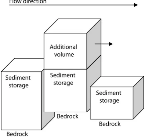
Therefore, both erosion and deposition can be simulated. If the calculated transport capacity exceeds the sediment in-put from the upstream section, erosion occurs as long as sedi-ment is available in the storage. Erosion is limited by the pre-defined depth of the sediment layer. The initial sediment vol-ume is defined by the depth of the sediment storage, which is a model input in each sub-grid cross-section. The actu-ally transported sediment is directed to the next downstream cross-section. If the sediment input into the section is larger than the transport capacity, deposition occurs and the sedi-ment storage is filled. During deposition it is possible that the river section becomes blocked and the discharge cannot flow through the section any more. This can especially occur at points with significant changes of the channel slope. If this problem occurs the additional volume that blocks the section is added to the next downstream cell (Fig. 4) and the slope is set to a predefined value of 0.1 %.

After each time step the slope of each cross-section is re-calculated according to the following formula in order to sim-ulate a mobile river bed:

S= hup−hdn ldn/2+lup/2+l

Fig. 4. Redistribution of additional sediment volumes in order to

avoid upward slopes.

wherehdn,hup are the downstream and upstream river bed

heights in m and ldn,up are the downstream and upstream

cross-section lengths in m. The newly defined slope is then used for transport simulations in the next time step.

4 The SETRAC model

In this study TOPKAPI is compared to the more so-phisticated specialised sediment transport model, Sediment TRansport in Alpine Catchments (SETRAC). SETRAC is briefly described here, focusing especially on the differences between the two models. SETRAC is a one-dimensional model for the simulation of sediment transport in torrents and mountain rivers and was developed at the University of Nat-ural Resources and Applied Life Sciences, Vienna (BOKU), Austria (Rickenmann et al., 2006; Chiari et al., 2010b). The model has been thoroughly tested against laboratory flume data and well documented field events by Chiari (2008) and Chiari and Rickenmann (2011). The channel network is rep-resented by nodes, cross-sections and sections. Nodes con-tain the information about the location of the related cross-sections. Cross-sections are described by pairs of points con-taining information about the distance from the left bank and the altitude. Each slice of the cross-section can be of the type main channel, bank or riparian. This discretization allows a detailed description of the cross-section geometry.

Erosion and deposition, as well as bedload transport can only occur in slices of the type main channel. Each cross-section contains information about the grain size distribution, the sediment storage depth and the initial slope. Input

hydro-graphs, simulated in HEC-HMS, can be assigned to cross-sections as time series. Sediment input as time series is also possible. For calculations, the cross-sections are connected by strips to get a representative discretization of the channel. The number of strips depends on the number of slices that are used to specify a cross-section, implying that the number of strips increases with the complexity of the cross-section. Dis-charge and bedload transport is calculated separately for each strip of the cross-section. The input hydrographs are routed using the kinematic wave approach that is solved numeri-cally by an explicit finite difference method with an upwind scheme. The same sediment transport equations as discussed in the previous section can be used in SETRAC, however SE-TRAC additionally allows for a fractional bedload transport. Feedback mechanisms of the changing river bed geometry on hydraulic simulations are possible, which is not the case in TOPKAPI. The interested reader is referred to Chiari (2008) and Chiari et al. (2010b) for more detailed descriptions of SETRAC.

5 Simulation of the 2005 event with TOPKAPI and SETRAC

The 2005 flood event in the Bernese Alps was taken as a case study to assess how the sediment transport module imple-mented in TOPKAPI compares to a dedicated and more so-phisticated model like SETRAC. This chapter describes the case specific settings of the models used for the simulations and presents the simulation results of both models. For the simulations, the Chiene as well as its most important tribu-tary Spigge have been considered. In total, 9.77 channel km have been simulated (8.24 km Chiene and 1.44 km Spigge). TOPKAPI has been forced with point information of the me-teorological input data temperature and precipitation taken from a meteorological station in Adelboden around 16 km in the South-West of the catchment, which were redistributed by means of appropriate lapse rates. The event duration of 60 h has been simulated using the geometrical information of Fig. 2c, the initial storage depths of Fig. 2b and the grain size distribution provided by Chiari et al. (2010b). 3600 sub-time steps have been taken for the temporal discretization of the sediment routing, which corresponds to a time step length of 1 s compared to 1 h for the hydrological simulations. An equal spacing between the sub-grids of 50 m has been as-sumed. The grid cell size is 250×250 m2.

a lumped rainfall-runoff model (Rickenmann and Koschni, 2010). However, we assume that the reconstructed and pub-lished values, provide at least an order of magnitude of dis-charge during the event which allows to assess the right order of magnitude of the simulated runoff. Simulations have been done for the entire year 2005 and initial conditions for the sediment simulations of the 60 h event have been taken from these simulations.

The same cross-sections as in SETRAC have been used for TOPKAPI and assigned to the corresponding raster cells. At the confluence point of Spigge and Chiene, one raster cell covers cross-sections of both rivers. It must be noted that the real confluence point is located further downstream with re-spect to the location identified in the model raster, which, due to the spatial resolution of the grid, locates the confluence point is slightly upstream. Thus, the simulated discharge of this raster cell represents already the merged rivers and is therefore much higher than the discharge of the Spigge cross-sections. In order to avoid overestimations of sediment transport capacities, the cross-sections of Spigge have been shifted upstream by one cell and the sediment output of the last Spigge cross-section is added to the correct cross-section of the Chiene. This modification allows for a more realistic simulation of the hydraulic conditions in the sub-grid cross-section.

The simulated hydrographs used as input to the SETRAC model have been also obtained by matching it to the recon-structed discharge in the different subcatchments. Thus, the 2005 event discharge simulations of both models compare very well, being this a prerequisite for the comparison of the sediment transport simulations. The 50 m spaced cross-sections used for the spatial discretisation every 50 m have been derived from the digital elevation model, which has been generated by airborne LiDAR before the extreme event occurred. It is worth noting that the sediment routine has no calibration parameter if it is used in the full transport capac-ity mode and only the exponentα can be changed to con-sider the effect of macro roughness. This parameter is global and cannot be optimised locally, e.g. at the sub-grid cross-section level. Stream channel parameters like width, slope, initial sediment storage are input data as well as sediment in-put from upstream and from major tributaries, and many of these parameters have to be derived or estimated from field observations.

The sediment transport simulations have been conducted in three different setups, M1 to M3, which differ by the se-lection of macro roughness equations (Table 1). The simula-tion results are presented in this chapter as a comparison of SETRAC and TOPKAPI. We also show reconstructed esti-mates of sediment transport volumes in order to demonstrate the credibility of the simulations. By the application to real data, though affected by errors and uncertainties difficult to quantify in the present case, we intend to show the ability of the scheme adopted in TOPKAPI to mimic a state of the art model for channel erosion and sediment transport, rather

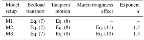
Table 1. Model setups of TOPKAPI and SETRAC used to simulate

the 2005 event. M3 was only used for TOPKAPI.

Model Bedload Incipient Macro roughness Exponent

setup transport motion effect α

M1 Eq. (7) Eq. (8) – –

M2 Eq. (7) Eq. (8) Eq. (11) 1.5

M3 Eq. (7) Eq. (8) Eq. (10) 1.5

than proving the ability of the model to reproduce the overall sediment balance during a storm event.

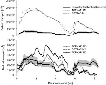
This is well illiustrated in Fig. 5, which shows a com-parison of SETRAC and TOPKAPI simulations with the ac-cumulated bedload transport recalculated from the morpho-logical changes. The time integrated bedload transport vol-umes are shown for the main channel (Chiene). The simula-tions of TOPKAPI and SETRAC with full transport capacity without any losses due to macro roughness or armour lay-ers (model setup M1) deliver comparable results but overes-timate the reconstructed bedload transport. TOPKAPI pro-duces slightly lower bedload transport than SETRAC espe-cially in the downstream part of the Chiene between 0.8 and 2 km. The contribution of the Spigge can be noticed at 6 km in the SETRAC simulations, whereas TOPKAPI only shows a minor reaction to these sediment inputs. In the upper parts of the Chiene both models deliver almost identical results. TOPKAPI simulations with higher critical discharges (not shown here), e.g. by using Eq. (9) instead of (8), are closer to the observed bedload transport, but in several sections no transport is simulated due to a too high incipient motion crite-ria. Considering an armour layer (Eq. 13) still lead to overes-timations of the observations by both models and compared to M1 there is only a small reduction of the total amount of bedload transported during the event (not shown here). It be-comes obvious that energy losses due to macro roughness are not negligible. These are considered in model setups M2 and M3 by means of two different equations butαalways equal to 1.5 (Fig. 5). Considering energy losses due to macro rough-ness delivers simulations closer to the observations. TOP-KAPI produces higher bedload transport than SETRAC if M2 is taken. M3 in TOPKAPI simulates discharge modified by Eq. (10) which is better suited for correction of high flow resistance with rectangular cross-sections because the water level as used in Eq. (11) depends more on the bed structure than the discharge. Equation (10) is not implemented in SE-TRAC.

6 Comparison of SETRAC and TOPKAPI

Fig. 5. Comparison of TOPKAPI, SETRAC and reconstructed bedload transport. The grey band indicates the±25 % error band. Simulations were done with different setups described in Table 1. A: Simulations with full transport capacity (M1), B: simulations considering losses due to macro roughness using setups M2 and M3. Note that Eq. (10) is not implemented in SETRAC and therefore M3 is only used for TOPKAPI simulations.

around 9 h for the simulations, whereas TOPKAPI needed 40 s. In SETRAC the strip-wise solution of the flow routing and bedload transport requires several iterations. The time step in SETRAC cannot be chosen by the user because the maximum allowed time step is calculated automatically to meet the Courant–Friedrichs–Lewy (CFL) stability criteria and is therefore not constant over the simulation time. Dur-ing high discharges the time step becomes very small (1.5 s for the presented case study). The time step for sediment routing in TOPKAPI is also small (1 s) but it is only applied on the sediment routing scheme and not on the hydraulic simulations. These are performed on the grid level with an hourly time step.

Figure 6 shows the transport capacities at 10, 30 and 60 h, the accumulated bedload transport, the channel reach slopes and the depth of the sediment storage at the respective time step. The transport capacities produced by TOPKAPI show less fluctuations than the ones by SETRAC. TOPKAPI gen-erally provides smaller transport capacities especially for the peaks at 3.5 and 7.0 km after 30 h. The variable slopes are comparable between the two models, however especially at the last time step SETRAC exhibits pronounced fluctu-ations of the simulated slopes, whereas TOPKAPI delivers smoothed slopes along the channel. The sediment storage

depths of TOPKAPI and SETRAC at 10 and 30 h corre-spond well. In the last time step, the sediment depths sim-ulated by TOPKAPI are more fluctuating between 1 and 2.5 km compared to SETRAC, and TOPKAPI also simulates an empty storage in the central part and upper reaches of the Chiene. SETRAC delivers fluctuating values between 0 and 1 m for these regions. A systematic difference be-tween the two model outputs can be observed at the con-fluence of the Spigge and the Chiene at 6.0 km. Although, the bedload transport simulations downstream and upstream of the confluence point are almost identical between the two models, the cross-sections that are directly affected by the confluence show significant differences. SETRAC delivers a much higher bedload transport and the sediment input from the tributary Spigge is clearly visible (peak at 6 km). TOP-KAPI only shows a very moderate reaction to the additional sediment input.

7 Discussion

Fig. 6. Detailed comparison of TOPKAPI and SETRAC for setup M1.

analyses is slope dependent (Scheidl et al., 2008) and in par-ticular more accurate for milder reaches. The mean vol-ume error can be determined by 0.3 m3m−2for the analysed catchment (Chiari et al., 2010a).

As expected, both models significantly overestimate sedi-ment transport if macro roughness is not taken into account. The simulated bedload transport is up to 10 times higher than the reconstructed transport. The comparison to the recon-structed bedload transport indicates that macro roughness re-sistance is probably non-negligible in modelling steep head-water streams. Literature confirms the importance of taking into account increased flow resistance due to macro rough-ness to obtain better agreement with observed and calculated bedload transport rates, e.g. Palt (2001), Rickenmann (2001, 2005), Rickenmann and Koschni (2010), Yager et al. (2007), Chiari and Rickenmann (2011). This can be explained by

Fig. 7. Comparison of SETRAC and TOPKAPI for the tributary Spigge. A: Accumulated discharge over the simulation period for each

cross-section element, B: accumulated transport capacity, C: bedload transport of each cross-cross-section of the entire simulation period, D: sediment storage depth of the last time step.

The comparison of the two models additionally revealed that differences can be observed at the confluence point of Spigge and Chiene. This is due to the spatial discretizations of the rivers on grid cell level and to differences in sediment transport simulations of the Spigge. In TOPKAPI the conflu-ence point of Spigge and Chiene and the lower cross-sections of Spigge are all covered by one grid cell which already holds the discharge contributions of the Spigge although on the sub-grid level the two rivers are still separated. The

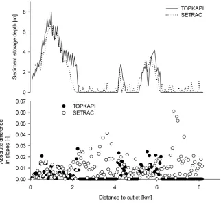
Fig. 8. Comparison of sediment storage depths and slope developments of SETRAC and TOPKAPI. A: Simulated sediment storage depths

by TOPKAPI and SETRAC for the last simulation time step; B: absolute differences between the bed rock slope and the slopes provided by TOPKAPI and SETRAC for the last simulation time step.

discharge at 0.8 km which is caused by a newly assigned hy-drograph at this cross-section (SETRAC is limited by the number of hydrographs that can be assigned to a simulation system). TOPKAPI simulates more stable but lower poten-tial transport rates, whereas SETRAC provides values almost three times higher than TOPKAPI (e.g. at 1.0 km in Fig. 7b). This causes an increased deposition simulated by TOPKAPI between the confluence point and 0.5 km (Fig. 7d). The sim-ulated sediment transport at the confluence point of Spigge and Chiene is more than double in SETRAC (Fig. 7c). There-fore, less sediment is provided to the river Chiene in the TOP-KAPI simulation, which is one reason for the lower sediment transport rates at the cross-sections downstream of the con-fluence point. However, the different sediment fluxes of the Spigge cannot explain the entire difference between the two models. Simulation results of TOPKAPI with the sediment fluxes taken from SETRAC as input to the Chiene river at the confluence point provide an improvement (not shown here) and the peak becomes more visible but TOPKAPI still deliv-ers bedload transport rates lower than SETRAC.

The fluctuations in SETRAC’s bed slope calculations are more pronounced at locations prone to bed erosion. TOP-KAPI simulates empty storages between 2.5 and 4.2 km and from 6.2 km upstream (Fig. 8a), whereas SETRAC still has

Fig. 9. Comparison of sediment transport simulations of TOPKAPI on the grid level with SETRAC. A: Simulated sediment storage depths

(with mobile and fixed beds); B: bedload transport without correction for high flow resistance.

Fig. 10. Effect of sub-time step modelling. A: Artificially redistributed sediment along the channel; B: accumulated, redistributed sediment

Table 2. Advantages and disadvantages of TOPKAPI and SETRAC.

TOPKAPI SETRAC

Advantages CPU time Detailed representation of channel cross-sections Direct coupling of hydrological and channel

processes

Graphical user interface with many visualization possibilities and geo-referenced representation of the channel network

Simulations at different spatial scales Internal discretization selectable by the user for sensitivity analysis

No selection of calculation time step required (model decides on the maximum allowed time step for stable calculation)

One grain model and fractional bedload transport calculations

Results can be stored as preformatted A0 DXF files for practical applications and as text files for detailed analysis

Disadvantages Only rectangular channel geometry CPU time Artificial redistribution in order to avoid

blocked channels

External simulations of the hydrology required

Limited to steep mountain rivers due to kinematic wave approximation No counter slopes or backwater effects considered

Limited to bedload transport (no suspended load or washload)

The efficiency of the sub-grid modelling technique in TOPKAPI becomes obvious if simulation results of sediment transport using the general grid level are compared to SE-TRAC (Fig. 9). To demonstrate this simulations with the M1 setup have been performed with the sub-grid procedure switched on and off, to mimic respectively a mobile (solid line in Fig. 9) and fixed (dashed line in Fig. 9) river bed. The geometrical information (width, initial slope and initial stor-age level) have been taken from the cross-sections which are covered by the respective grid cells as mean values. Also in the case with inactive sub-grid the basic pattern of the SE-TRAC bedload transport simulations is reproduced (Fig. 9b), however lower transport rates are simulated. Interestingly, the model run with a fixed bed slope provides sediment trans-port rates closer to SETRAC than the one with variable bed slope especially between 0 and 5 km. However, the storage heights do not agree well with the SETRAC results (Fig. 9a). This shows that for a first assessment sediment transport sim-ulations using the grid level can already provide estimates of acceptable reliability, especially considering the significantly low required amount of geometrical information. However, the overall comparison shows that the sub-grid modelling scheme significantly improves the simulation results, espe-cially when sediment storage depths (Figs. 6 and 8a) and the slope evolution (Fig. 6) are considered.

It is finally interesting to discuss the effect of the sub-time step modelling, which is shown in Fig. 10. In order to avoid the blocking of the channel the model operates a redistribu-tion of the sediment (see Sect. 2.3.2 above for details). The relative number of redistributions in Fig. 10a, i.e. the total number of artificial redistributions divided by the total num-ber of time steps (numnum-ber of sub-time steps ×number of global time steps), shows that the artificial redistribution of additional sediment volumes significantly reduces with in-creasing number of sub-time steps. With smaller time steps (e.g. 1 s), the transported sediment volume per time step is smaller than with larger time steps (e.g. 1 h), thus the chance of blocking the channel is smaller when using the mobile bed approach, which adjusts the slopes at the end of each time step. Interestingly, the redistributed sediment volumes in Fig. 10b already converge at a relatively small number of sub-time steps, n, and n=7 (equivalent to a time step of 514.3 s) provides a total redistribution volumes comparable to that obtained for n=3600 (equivalent to a time step of 1 s). Thus the artificial redistribution can be minimized by a sufficiently small sub-time step.

8 Conclusions and outlook

and continuous in time hydrological model TOPKAPI en-ables the simulation of sediment transport rates, erosion and deposition patterns and bed slope developments in a river channel network. This implementation offers new and inter-esting perspectives to model erosion and sediment transport across an entire catchment, not only throughout one storm rainfall event, but also over longer terms, with results that are comparable to specialised models based on computation-ally demanding hydraulic schemes. Thus, since the transport module is directly coupled to the hydrological model, effects of changes in the hydrological cycle on the sediment trans-port patterns can be studied.

The performance of the sediment transport accounting TOPKAPI compared to a more sophisticated, specialised sediment transport model (SETRAC) is satisfying. The ad-vantages and disadad-vantages of the two models are summa-rized in Table 2. The major innovation of this study is the implementation of the sub-grid modelling scheme, which significantly improves the simulation of the bedload sedi-ment transport compared to the coarser grid level simulation. The assumption that discharge can be simulated at the grid level and used for all sub-grid sections within that grid cell provides reliable sediment discharge simulations. This ap-proach exhibit inaccuracies at confluence points, for which a more sophisticated solution for flow partitioning should be used based on the ratio of inflowing discharge from the up-stream cells.

At the present stage of development TOPKAPI does not consider yet a feedback mechanism of the mobile bed on the hydraulic simulations. This limitation can be reasonable if the slope changes are moderate during an event. How-ever, an up-scaling of the sub-grid geometry to account at the model general grid level for changes induced by ero-sion and sediment transport should be investigated further. Moreover, we have shown that sediment transport simula-tions in the modified TOPKAPI are computationally quite efficient, since the model requires only 40 s on a standard desktop computer for the simulation of the 60 h event with 3600 internal sub-time steps, especially when compared to an equally performing specialised model requiring a thou-sand times longer simulation.

Finally, while we recognise that the model requires to be further validated on additional real events, we believe that the study shows a direction in which integrated models, which combine the modelling of catchment hydrological response and of processes driven by it, can evolve. Recent floods in several mountain regions of Switzerland and Europe have shown that there is indeed an impelling need, both for de-sign purposes and in real-time, of models that can efficiently simulate across different catchment scales the multiple ef-fects of storm rainfall, such as the serial dependence of soil slips, diffused erosion and channel sediment transport. The sediment accounting TOPKAPI model, which has been pre-sented in this study, aims at tracing a path that can cover that need.

Acknowledgements. We highly acknowledge the inputs and dis-cussions of Francesca Pellicciotti. This study has been carried out within the project APUNCH (Advanced Process UNderstanding and prediction of hydrological extremes and Complex Hazards) funded by the Competence Center Environment and Sustainability (CCES) of the ETH Domain (Switzerland).

Edited by: J. Freer

References

Bahadori, F., Ardeshir, A., and Tahershamsi, A.: Prediction of allu-vial river bed variation by SDAR model, J. Hydraulic Res., 44(5), 614–623, 2006.

Badoux, A. and Rickenmann, D.: Berechnung zum Geschiebetrans-port w¨ahrend der Hochwasser 1993 und 2000 im Wallis, Wasser Energie Luft, 3, 217–226, 100. Jahrgang, 2008 (in German). Bathurst, J. C., Li, R.-M., and Simons, D. B.: Resistance equation

for large-scale roughness, J. Hydr. Div., 107, 1593–1613, 1981. Beffa, C.: 2D-Simulation der Sohlenreaktion in einer

Flussverzwei-gung, ¨Osterreichische Wasser- und Abfallwirtschaft, 42(1–2), 1– 6, 2005 (in German).

Chiari, M.: Numerical modelling of bedload transport in torrents and mountain streams. PhD dissertation, University of Natural Resources and Applied Life Sciences, Vienna, Austria, 2008. Chiari, M. and Rickenmann, D.: Back-calculation of bedload

trans-port in steep channels with a numerical model, Earth Surf. Pro-cess. Landforms, 36, 805–815, doi:10.1002/esp.2108, 2011. Chiari, M., Scheidl, C., and Rickenmann, D.: Assessing

morpho-logic changes caused by torrential flood events with airborne lidar data, in: Global Change – Challenges For Soil Manage-ment, Adv. Geoecol., 41, 192–202, Catena Verlag, ISBN: 978-3-923381-57-9, 2010a.

Chiari, M., Friedl, K., and Rickenmann, D.: A one dimensional bedload transport model for steep slopes, J. Hydraul. Res., 48(2) 152–160 doi:10.1080/00221681003704087, 2010b.

Corripio, J. G.: Vectorial algebra algorithms for calculating terrain parameters from DEMs and solar radiation modelling in moun-tainous terrain, Int. J. Geogr. Inf. Sci., 17(1), 1–23, 2003. Deyhle, C., Glugla, G., Golf, W., v. Hoyningen Huene, J., Kalweit,

H., Olbrisch, H., Richter, D., Wendling, U., Wessolek, G., and Wittenberg, H.: Ermittlung der Verdunstung von Land- und Wasserfl¨achen. Technical Report 238, Deutscher Verband f¨ur Wasserwirtschaft und Kulturbau e.V. (DVWK), 1996.

Doten, C. O., Bowling, L. C., Lanini, J. S., Maurer, E. P., and Lettenmaier, D.,P.: A spatially distributed model for the dy-namic prediction of sediment erosion and transport in moun-tainous forested watersheds, Water Resour. Res. 42, W04417, doi:10.1029/2004WR003829, 2006.

Fehr, R.: A method for sampling very coarse sediments in order to reduce scale effects in movable bed models. Proc. Symp. Scale effects in modelling sediment transport phenomena, Toronto, IAHR, Delft, 383–397, 1986.

Hassan, M. A., Church, M., and Lisle, T. E.: Sediment transport and channel morphology of small, forested streams, J. Am. Water Resour. Assoc. 41(4), 853–876, 2005.

Khorram, S. and Ergil, M.: Most Influential Parameters for the Bed-Load Sediment Flux Equations Used in Alluvial Rivers, J. Am. Water Resour. As., 46(6), 1065–1090, 2010.

Liu, Z. and Todini, E.: Towards a comprehensive physically-based rainfall-runoff model, Hydrol. Earth Syst. Sci., 6, 859–881, doi:10.5194/hess-6-859-2002, 2002.

Liu, Z., Martina, M. L. V., and Todini, E.: Flood forecasting using a fully distributed model: application of the TOPKAPI model to the Upper Xixian Catchment, Hydrol. Earth Syst. Sci., 9, 347– 364, doi:10.5194/hess-9-347-2005, 2005.

Lokale l¨osungsorientierte Ereignisanalyse (LLE) Reichenbach. In Technischer Bericht. Emch + Berger AG, Spiez; Hunziker, Zarn & Partner AG, Aarau; Geotest AG, Zollikofen. Tiefbauamt Kan-ton Bern, Bern, unpublished, 2006 (in German).

Mathys, N., Brochot, S., Meunier, M., and Richard, D.: Erosion quantification in the small marly experimental catchments of Draix (Alpes de Haute Provence, France): Calibration of the ETC rainfall-runoff-erosion model, Catena, 50, 527–548, 2003. MeteoSchweiz: Starkniederschlagsereignis August 2005.

Arbeits-berichte der MeteoSchweiz 211, Bundesamt f¨ur Meteorologie und Klimatologie, 63 pp., 2006.

Meyer-Peter, E. and Mueller, R.: Formulas for bedload transport, 2nd IAHR Congress,. Stockholm, Appendix 2, 39–64, 1948. Nitsche, M., Rickenmann, D., Turowski, J., Badoux, A., and

Kirchner, J.: Evaluation of bedload transport predictions us-ing flow resistance equations to account for macro-roughness in steep mountain streams, Water Resour. Res., 47, W08513, doi:10.1029/2011WR010645, 2011.

Palt, S.: Sedimenttransporte im Himalaya-Karakorum und ihre Bedeutung f¨ur Wasserkraftanlagen, Mitteilung 209, Institut f¨ur Wasserwirtschaft und Kulturtechnik, Universit¨at Karlsruhe, Karlsruhe Germany, 2001 (in German).

Papanicolaou, A., Bdour, A., and Wicklein, E.: One-dimensional hydrodynamic/sediment transport model applicable to steep mountain streams, J. Hydraulic Res., 42(4), 357–375, 2004. Pellicciotti, F., Brock, B., Strasser, U., Burlando, P., Funk, M., and

Corripio, J.: An enhanced temperature-index glacier melt model including the shortwave radiation balance: development and test-ing for Haut Glacier d’Arolla, Switzerland, J. Glaciol., 51(175), 573–587, 2005.

Recking, A., Frey, P., Paquier, A., Belleudy, P., and Champagne, J. Y.: Feedback between bed load transport and flow resist-ance in gravel and cobble bed rivers, Water Resour. Res., 44, W05412, doi:10.1029/2007WR006219, 2008.

Reichel, G., F¨ah, R., and Baumhackl, G.: FLORIS-2000: Ans¨atze zur 1.5D Simulation des Sedimenttransportes im Rahmen der mathematischen Modellierung von Fließvorg¨angen, in: Internat, Symposion “Betrieb und ¨Uberwachung wasserbaulicher Anla-gen”, 2000 (in German).

Rickenmann, D.: Bedload transport capacity of slurry flows at steep slopes. Mitteilung, 103, Versuchsanstalt f¨ur Wasserbau, Hydrolo-gie GlazioloHydrolo-gie, ETH Zurich, Zurich, 1990.

Rickenmann, D.: Hyper-concentrated flow and sediment transport at steep slopes, J. Hydraul. Eng., 117(11), 1419–1439, 1991. Rickenmann, D.: An alternative equation for the mean velocity in

gravel-bed rivers and mountain torrents, Proc. Nat. Conf. Hy-draulic Engineering, Buffalo NY 1, 672–676, editd by: Cotro-neo, G. V. and Rumer, R. R., ASCE, New York, 1994.

Rickenmann, D.: Fliessgeschwindigkeit in Wildb¨achen und Gebirgsfl¨ussen, Wasser, Energie, Luft., 88(11/12), 298–304, 1996 (in German).

Rickenmann, D.: Comparison of bed load transport in torrents and gravel bed streams, Water Resour. Res. 37(12), 3295–3305, 2001.

Rickenmann, D.: Geschiebetransport bei steilen Gef¨allen. Mit-teilung 190, 107–119. Versuchsanstalt f¨u r Wasserbau, Hydrolo-gie und GlazioloHydrolo-gie, ETH Zurich, Zurich, 2005 (in German). Rickenmann, D., Chiari, M., and Friedl, K.: SETRAC – A

sedi-ment routing model for steep torrent channels. River Flow 2006 1, 843–852, edited by: Ferreira, R., Leal, E. A. J., adn Cardoso, A., Taylor & Francis, London, 2006.

Rickenmann, D. and Koschni, A.: Sediment loads due to fluvial transport debris flows during the 2005 flood events in Switzer-land, Hydrol. Process, 24, 993–1007, 2010.

Rinderer, M., Jenewein, S., Senfter S., Rickenmann, D., Sch¨oberl, F., St¨otter, J., and Hegg, C.:. Runoff and bedload transport modelling for flood hazard assessment in small alpine catchments -the PROMAB-GIS model, in: Sustainable Natural Hazard Man-agement in Alpine Environments, edited by: Veulliet, E., St¨otter, J., and Weck-Hannemann, H.. Springer, Heidelberg, New York, 69–101, 2009

Scheidl, C., Rickenmann, D., and Chiari, M.: The use of airborne LiDAR data for the analysis of debris flow events in Switzerland, Nat. Hazards Earth Syst. Sci., 8, 1113–1127, doi:10.5194/nhess-8-1113-2008, 2008.

Todini, E. and Ciarapica, L.: The TOPKAPI model, in: Mathemati-cal models of large watershed hydrology, edited by: Singh, V. P., Water Resources Publications, Littleton, Colorado, USA, 2001. Todini, E. and Mazzetti, C.: TOPKAPI User manual and references,

PROGEA, 2008.

Wicks, J. M. and Bathurst, J. C.: SHESED:Aphysically based, dis-tributed erosion and sediment yield component for the SHE hy-drological modelling system, J. Hydrol., 175, 213–238, 1996. Yager, E. M., Kirchner, J. W., and Dietrich, W. E.: Calculating bed