Estimation of high return period flood quantiles using additional non systematic information with upper bounded statistical models

www.hydrol-earth-syst-sci.net/14/2617/2010/ doi:10.5194/hess-14-2617-2010

© Author(s) 2010. CC Attribution 3.0 License.

Earth System

Sciences

Estimation of high return period flood quantiles using additional

non-systematic information with upper bounded statistical models

B. A. Botero1and F. Franc´es2

1_{Facultad de Ingenier´ıa y Arquitectura, Universidad Nacional de Colombia, Sede Manizales, Colombia} 2_{Instituto de Ingenier´ıa del Agua y Medio Ambiente, Universidad Polit´ecnica de Valencia, Valencia, Spain} Received: 19 June 2010 – Published in Hydrol. Earth Syst. Sci. Discuss.: 5 August 2010

Revised: 20 November 2010 – Accepted: 29 November 2010 – Published: 20 December 2010

Abstract. This paper proposes the estimation of high re-turn period quantiles using upper bounded distribution func-tions with Systematic and additional Non-Systematic infor-mation. The aim of the developed methodology is to reduce the estimation uncertainty of these quantiles, assuming the upper bound parameter of these distribution functions as a statistical estimator of the Probable Maximum Flood (PMF). Three upper bounded distribution functions, firstly used in Hydrology in the 90’s (referred to in this work as TDF, LN4 and EV4), were applied at the Jucar River in Spain. Dif-ferent methods to estimate the upper limit of these distribu-tion funcdistribu-tions have been merged with the Maximum Likeli-hood (ML) method. Results show that it is possible to ob-tain a statistical estimate of the PMF value and to establish its associated uncertainty. The behaviour for high return pe-riod quantiles is different for the three evaluated distributions and, for the case study, the EV4 gave better descriptive re-sults. With enough information, the associated estimation uncertainty for very high return period quantiles is consid-ered acceptable, even for the PMF estimate. From the ro-bustness analysis, the EV4 distribution function appears to be more robust than the GEV and TCEV unbounded distri-bution functions in a typical Mediterranean river and Non-Systematic information availability scenario. In this scenario and if there is an upper limit, the GEV quantile estimates are clearly unacceptable.

Correspondence to: F. Franc´es ([email protected])

1 Introduction

Flood frequency analysis is one of the most common meth-ods to estimate the design flood for hydraulic structures and for flood hazard/risk mitigation programs. In Europe, the na-tional legislation for flood risk assessment is based on flood frequency analysis to estimate discharges associated with dif-ferent return periods, from 50 to 500 years (Benito et al., 2004). In some projects the focus is on extreme floods, which have been defined according to different authors as floods with an annual probability of occurrence of about 10−3 _to 10−7_{(Jarret and Tomlinson, 2000), 10}−3_{or lesser} (Naghet-tini et al., 1996) and in other cases, as floods with return periods greater than 500 years (England et al., 2003). Tra-ditionally, extreme flood estimates have been associated with large dam projects or with the location of nuclear and other high vulnerable facilities, in which the release of hazardous materials to the environment is in consideration (Stevens, 1992). For some of these projects, the design criteria com-monly include the Probable Maximum Flood (PMF) estima-tion. The PMF is the biggest flood physically possible at a specific catchment (Smith and Ward, 1998). It has a phys-ical meaning and it provides an upper limit of the interval within which the decision maker must operate and design. The PMF is the flood generated by the Probable Maximum Precipitation (PMP) with the worst but reasonable hydrologi-cal conditions in the studied basin. The PMP is defined by the World Meteorological Organization as a precipitation upper limit for a given region, duration and time of the year (WMO, 1986).

Systematic information). This fact involves the extrapola-tion of very high return period quantiles from data records which rarely exceed a hundred of years, producing quantile estimates with a high level of uncertainty.

In the last decades, as a way to solve this problem, many authors have included historic and palaeoflood information (from now, Non-Systematic information) in flood frequency analysis with very good results: starting from the pioneer pa-per of Leese (1973) and following by the work of Stedinger and Cohn (1986), Hosking and Wallis (1986a,b), Stedinger and Baker (1987), Jin and Stedinger (1989), Stevens (1992), Pilon and Adamowski (1993), Frances et al. (1994), Cohn et al. (1997), Jarret and Tomlinson (2000), Martins and Ste-dinger (2001), O’Conell et al. (2002), England et al. (2003), Naulet et al. (2005), Reis and Stedinger (2005) and Merz and Bl¨oschl (2008).

Probability distribution functions with 2, 3 or 4 param-eters have been used in extreme floods frequency analysis with the common characteristic of having no upper bound, at least for high positive skewness coefficient (γx). The use of parametric distribution functions allows the quantile extrap-olation as a function of the requested return period as much as it is required (obviously increasing at the same time its uncertainty). However, as the return period increases with unbounded parametric distribution functions, the estimated quantiles increase too with no limit. Though, the question to pose at this point is: would it be possible to have a flood with such a high magnitude, as large as it could be obtained with these unbounded distribution functions, for a certain catchment with specific area and geomorphologic character-istics? The straight answer is no, this is not possible. There must be a limiting flood discharge which is the biggest phys-ically possible flood for the specific climatic and hydrologic characteristics of the catchment, which indeed corresponds with the PMF definition (Enzel et al., 1993). Or in Horton’s words: “... a small stream cannot produce a major Missis-sippi flood for much the same reason a barnyard fowl cannot lay an egg a yard in diameter” (second author’s class notes of J. Salas’ lecture in 1990). Not considering the existence of this upper limit must introduce an additional significant model error in the high return period estimated quantiles. Moreover, in our opinion, this additional error could produce in most cases the underestimation of the high return period quantiles, which is one of the most frequent causes of dam failure (ASCE, 1988).

In accordance with reality, some distribution functions in-corporate an additional parameter, which is actually the up-per limit to the random variable. This class of functions has been applied to the extreme frequency analysis of annual maximum daily precipitation by El´ıasson (1994 and 1997), Takara and Loebis (1996) and Takara and Tosa (1999) and in frequency analysis of annual maximum flood by Takara and Tosa (1999). All these authors concluded that upper bounded distribution functions fit properly to extreme data and im-prove the quantile estimates.

In this paper we propose the use of upper bounded distri-bution functions, in order to better estimate high return pe-riod quantiles. The upper limit of these distribution func-tions can be fixed a priori or not. Following the classification of Merz and Bl¨oschl (2008) for additional information, in the first case the PMF value can be considered as a causal information expansion. This was the option followed pre-viously by El´ıasson (1997), Takara and Loebis (1996) and Takara and Tosa (1999). In the last case, the PMF can be estimated as one of the parameters of the statistical model, using in this paper additional Non-Systematic information, called temporal information expansion, in terms of Merz and Bl¨oschl (2008) to obtain enough estimation reliability.

2 Upper bounded distribution functions

If parent distribution is upper bounded, the annual maximum will also be. In this situation, upper unbounded classical lim-iting functions from Extreme-Value Theory will not be good approximations for the estimation of high return period an-nual maximum, as it will be shown in the robustness analysis in Sect. 6. The three upper bounded distribution functions applied in the case study were chosen because they had been previously successfully applied to hydrological extremes se-ries. Other distribution functions commonly used in Hydrol-ogy which have an upper bound are the Generalized Pareto and the GEV. The former has an upper bound when its shape parameter is bigger than 0, which occurs forγx<2.0. The latter presents an upper bound when the shape parameter is also positive, but then, γx becomes less than the Gum-bel’s constant skewness coefficient, which is equal to 1.14. Our aim is to analyse rivers with high skewness coefficient (γx clearly bigger than 2), like those with a Mediterranean regime, which is the reason to not include in this paper the GEV and Generalized Pareto distribution functions.

Following paragraphs presents a short description con-cerning the three selected distributions. More behavioural and statistical details can be found in Botero (2006). 2.1 The extreme value with four parameters

distribution function (EV4)

This probability distribution function was firstly proposed by Kanda (1981), who empirically derived it from the EV dis-tribution function family. The EV4 cumulative disdis-tribution function (cdf) is given by

FX(x) = exp

"

−

_{g −x}

ν (x −a)

k#

(1)

k > 0; v > 0; a ≤ x ≤ g

Takara and Tosa (1999) applied this distribution to annual maximum daily precipitation and annual maximum daily dis-charge at Ohtsu (Japan). The authors made a sensitivity anal-ysis fixing the upper and lower bounds to a priori values ob-tained empirically. They concluded in a comparison with other distribution functions, the EV4 is the most appropri-ated to datasets with sample skewness coefficient higher than about 2.

2.2 The Slade-type four parameter LogNormal distribution function (LN4)

Proposed by Slade (1936) and named in this manner by Takara and Loebis (1996), the LN4 can be obtained if a Slade-type random variable transformation is applied to a Two Parameters LogNormal distributed random variable. This transformation is given by

y = ln

_{x −a}

g −x

a ≤ x ≤ g (2)

wheregandaare respectively the upper and lower bounds. The resulting LN4 pdf is defined as following

fX(x) =

g −a (x −a) (g −x) σy

√

2π (3)

exp

"

−1

2

_{y −µ}

y

σy

2#

whereµyandσyare the well known LogNormal cdf param-eters. From the LN4 application to annual maximum daily precipitation data, Takara and Loebis (1996) concluded that if the four parameters of the distribution are estimated, the variability of quantile estimates is higher than if one or both limits are fixed previously in a known value. In addition, they suggested the use of the PMF as the upper bound when deal-ing with floods. In a posterior paper, Takara and Tosa (1999) conclude that the LN4 distribution function fits well to many hydrological datasets with sample skewness coefficient less than about 1.5.

2.3 The transformed extreme value type distribution function (TDF)

This distribution was proposed by El´ıasson (1994) as a sta-tistical model for frequency analysis of extreme precipita-tion. The author suggested that bounded data fitted by an unbounded distribution as the EV1 (also called Gumbel), must deviate from the distribution at high return periods. In El´ıasson (1997) is defined a Transformed Distribution Func-tion (TDF) derived from a Base DistribuFunc-tion FuncFunc-tion (BDF) selected by the author, which corresponds with the EV1. In his work, El´ıasson (1997) fits the resulting TDF to standard-ized annual maximum daily precipitation from Iceland and Washington State (USA) with very good results fixing a prior

estimate of the PMP. The final expression of the TDF cdf is given by

FX(x) = exp

−exp

₋

x

α +

α k∗ (g −x) −b

(4)

α > 0; k∗ < 0 and x ≤ g

wheregis the upper bound, αis a scale parameter, b is a location parameter, andk∗is a negative constant.

3 Parameter estimation methodology

3.1 Maximum Likelihood method and data classification

In this study, the parameters set for each distribution func-tion is estimated based on the Maximum Likelihood (ML) estimation method, as in many others works dealing with Non-Systematic information (Leese, 1973; Condie and Lee, 1982; Hosking and Wallis, 1986; Cohn and Stedinger, 1987; Phien and Fang, 1989; Guo and Cunnane, 1991; Pilon and Adamowski, 1993; Frances et al., 1994; Kroll and Ste-dinger, 1996; Frances, 1998; Martins and SteSte-dinger, 2001; O’Connell et al., 2002; Williams, 2002; Naulet et al., 2005; Calenda et al., 2005; Calenda et al., 2009). This methodol-ogy has been selected on the basis of its statistical features for large samples, and also because of its ability to incorpo-rate easily in the estimation process any type of additional data.

palaeoflood information) or the minimum discharge which produces damages in a city (for historical information). It can change with time and, in some cases, there can be upper and lower thresholds for the same flood (following the palae-oflood example if there are two caves at different positions, the lower one with sediments of a particular flood and the up-per one without any trace of this flood). On the other hand, usually the Systematic data is completely known, but some times the uncertainty in the data forces to treat them also as censored.

Concerning “years without information” within the Non-Systematic period, the statistical treatment depends on the situation. If there is no information during some years (his-torical or palaeoflood), it will be in the major part of the cases because the flood was below the threshold level of perception and, therefore, they must be considered as UB data. If “we do not know what happened”, the solution is the same than we traditionally do when dealing with the Systematic record: do nothing and assume there is not a bias to miss the very high floods or very low ones. But the last situation should be very rare, because very frequently there is more than one source of information. For example, palaeoflood studies look for slackwater deposits in more than one location, in order to reduce the possibility of missing floods over the threshold level of perception.

Stedinger and Cohn (1986) and Frances et al. (1994) first classified the flood information from a statistical point of view. However, in a Maximum Likelihood framework, our experience dictates it is more convenient to follow the classi-fication presented by Naulet (2002), in which any piece (Sys-tematic or Non-Sys(Sys-tematic) of flood data can be classified in (see Fig. 1):

– EX type. The flood peak value is known. It will corre-spond with most of the Systematic data and with some Non-Systematic floods with enough information to re-construct the peak discharge.

– LB type. In this case, it is only known that the flood was bigger than a lower boundL, which is the knownXH. – UB type. For this type of data it is known that at the time

of the flood, an upper bound (U) with known magnitude was not exceeded. Again, thisU corresponds with the

XH.

– DB type. The flood peak is unknown and the only in-formation about this flood is that it has a double bound. This means that the flood was within an interval with known values for the upper (U) and lower (L) bounds. For annual maxima analysis of a stationary process, but with variable threshold of perception in time, depending on the type of data each yearicontributes to the likelihood function through one of these general expressions:

LSY(2;x) = fX xi;2

(5)

time

d

is

c

h

a

rg

e

XH

Known flood discharge

Unknown flood discharge

DB

LB

UB

EX

XH1 XH2

Threshold level of perception

Fig. 1. Proposed flood data classification (after Naulet, 2002), in this figure with two constantX_H.

LLB,i 2;Li = 1 −FX Li;2 (6)

LUB,i 2;Ui = FX Ui;2 (7)

LDB,i 2;Li, Ui =FX Ui;2 −FX Li;2 (8) where the independent and identically distributed random variableXis described for all years through its probability density functionfX(·)or its cumulative distribution function

FX(·);2represents the parameters set;xi is the magnitude of the flood presented in thei-year; Ui is the upper bound which is not exceeded in the i-year; and Li is the lower bound exceeded in thei-year. The ML estimated parameters are obtained by maximizing the logarithm of the likelihood function over the parameter space.

When dealing with Non-Systematic information, what is commonly available is a combination of the different types of data described above, as it is shown in Eq. (13) for the like-lihood function of the case study (Sect. 4). It was stressed by Frances et al. (1994), that from the statistical point of view there is no difference concerning the source of the Non-Systematic information, historical or palaeoflood, and their treatment must be completely similar. More over, with this new data classification there is not any difference also be-tween Systematic and Non-Systematic information, with the additional advantage that always the data can have a time as-signed, which will be crucial for future non-stationary flood frequency models.

3.2 Upper limit estimation

El´ıasson (1997) and Takara and Loebis (1996). In this case,

Gis the PMF estimate by traditional means. The PMF can be estimated by different procedures, being the most advis-able the rainfall-runoff modelling, where rainfall input is the PMP estimated by the WMO maximization and transposition procedure (WMO, 1986).

A second possibility is to estimate the whole parameters set, includingg, using the ML method. However, with EV4 and TDF distribution functions and when the available Non-Systematic information is a mix of EX and UB data (also called Censored Information or CE by Stedinger and Cohn, 1986), the estimated gˆ is equal to the maximum observed value of the data set (which obviously it is not the PMF) and thus, other methods to estimategmust be introduced. This follows from the fact that the likelihood function for these two distributions and this type of information decreases monotonically forg→ ∞(Kijko and Sellevoll, 1989).

Kijko (2004) proposed what he called a “Generic Equa-tion” (GE) for the estimation of the maximum earthquake magnitude, which corresponds with the magnitude of the largest possible earthquake, conceptually equivalent to the PMF for floods. This author developed this equation based on the limit of a random variable estimator proposed by Cooke (1979). The GE is valid for any cdf and it is given by

g = xmax+ g

Z

−∞

FX(x;2)

n

dx (9)

wherexmaxis the maximum observed value of the Systematic and Non-Systematic data, andnis the number of observed values (i.e., thexmaxorder). It must be noticed that it is not possible to apply the Generic Equation when there are LB or DB data in the available information, because with this kind of data thexmaxorder cannot be known.

3.3 Proposed estimation methodologies

In this paper and in accordance with the selected method to estimateg, the whole parameters set estimation method will be referred as following

ML-C: When the whole parameters set of the distribution function is estimated by the ML method, includinggas an-other free parameter in the maximization process:

maxL(2) (10)

ML-GE: It will be referred to the Maximum Likelihood-Generic Equation estimation method. This method consists on the use of the Generic Equation presented above (Eq. 9) to estimategand the ML method for the rest of parameters:

maxL(20) g = xmax +

g

R

−∞

FX(x;20, g)

n

dx

 



(11)

where20is the parameters set excludingg. The expression in Eq. (11) must be solved iteratively, fixing thegwhen max-imizing the likelihood function and fixing the rest of parame-ters when obtaining a newgvalue with the Generic Equation. This procedure is repeated until the estimatedg converges with the proper tolerance.

ML-PG: Finally, in this case, gis fixed at the value previ-ously calculated (G) as the best approximation for the true unknown PMF, and the other parameters are estimated by ML method:

g = G

maxL(20)

(12)

4 The Jucar River case study

The statistical models described above have been applied to the available data of the Jucar River at “Huerto-Mulet” flow gauge station, where we had Systematic annual maximum flows from 1946 to 2004 (56 years). This river is located in a semi-arid climate region of Eastern Spain and has a long period with historical information. The point of interest is close to the river sea mouth and has a basin of 21 500 km2, but due to meteorological reasons, actually only one third of the basin is contributing to the floods in this area. The basin mean annual precipitation is 450 mm, but it must be under-lined that the Jucar River presents the typical high variabil-ity (or torrentiallvariabil-ity) of Mediterranean rivers, with frequent observed daily precipitation events with more than 100 mm during the Fall season. These extreme events are generated by strong Convective Mesoscale Systems positioned in the Western Mediterranean Sea (Rigo and Llasat, 2007). The main sample statistical characteristics of the instantaneous annual maximum floods are: mean = 713 m3s−1, coefficient of variation = 2.74 and skewness coefficient = 5.26.

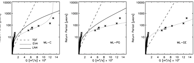
Fig. 2. Applied models to the Jucar River. Stars are the sample plotting positions given by theEformula. Triangle represents theXH= 6200 m3s−1plotting position. Figures correspond to each estimation method: ML-C (left), ML-PG (central) and ML-GE (right).

with a flood of 12 000 m3s−1, and it was almost exceeded in 1987 with a flood of 5200 m3s−1. The stationarity of this long information period (more than 200 years) was tested and proved with the test of stationarity described by Lang et al. (1999 and 2004), using as random variable the cumula-tive number of floods over the threshold of perception. As an example of application of Eqs. (5) to (8), the likelihood function for this case study is:

L(2) =

FX(6200;2) 150

(13) 3

Y

i=1

fX yi;2 56

Y

i=1

fX xi;2

where the first term represents the contribution to the like-lihood function of the Non-Systematic UB floods (during the Non-Systematic period the annual maximum flood did not reach the convent 150 years), theyi are the three Non-Systematic EX floods and thexiare the Systematic ones.

Franc´es (1998) studied this case study, using the un-bounded distribution function TCEV, which assumes a mixed population of “ordinary” and “extraordinary” flood events (Rossi et al., 1984), the later originated by Convective Mesoscale Systems. In this work, the statistical models ap-plied for the flood frequency analysis of the Jucar River are combinations of the three bounded distribution functions pre-sented in Sect. 2 and the three parameter estimation methods shown in Sect. 3. The lower bound for the EV4 and LN4 has been fixed to zero, hence reducing to three the number of pa-rameters to be estimated. In any case, this is not an influential parameter for high return period quantiles.

In order to apply the ML-PG parameter estimation method, a previous PMF value to the Jucar River catchment must be calculated. Cifres and Abad (1992), using for the PMP the maximization and transposition procedure (WMO, 1986), computed the PMF in 25 000 m3s−1for the Tous dam, which is located upstream our point of interest. Assuming the same specific discharge (overestimating hypothesis), tak-ing into account the catchment area increment and consid-ering only the meteorologically active basin, the PMF can be extrapolated to 33 900 m3s−1at Huerto-Mulet flow gauge

station. With a high probability, it will be an overestimation of the PMF. With any better estimation, due to the scope of this study, this value will be used forG.

Usually, to test the model performance (distribution and estimation method) from a “descriptive” point of view (Cun-nane, 1986), the fitted cdf and the plotting positions are com-pared graphically. In this work, the probability plotting po-sitions with Systematic and CE Non-Systematic information were calculated with theEformula proposed by Hirsh and Stedinger (1987). Figure 2 shows the plotting positions for the Jucar data and the fits of the applied distribution functions by each parameter estimation method.

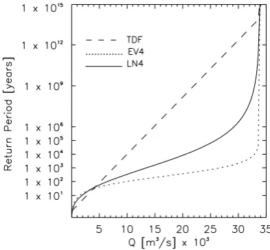
A very interesting first conclusion about the three upper bounded distribution functions is their completely different behaviour approaching the upper limit: the EV4 do it faster than the LN4 and the TDF is the slowest, even if the upper limit is the same as in Fig. 2b or, better, in Fig. 3 (which is a more general view of Fig. 2 (central), including the same upper limit). This different behaviour can be generalized for the usual parameter range of the three functions and results in most cases crucial for the model selection.

For the Jucar sample data, Fig. 2 shows the characteris-tic “dog-leg” effect in torrential regime rivers. It is clear the TDF distribution can not reproduce the shape of the plot-ting positions. The reason for this unsuitability could be that the TDF is based on a Gumbel distribution function, which, according to Franc´es (1998), is not appropriate for Mediter-ranean rivers. On the other hand, the EV4 distribution func-tion with all the parameter estimafunc-tion methods is the cdf that better reproduces the shape of the plotting positions. The tri-angle in Fig. 2 represents the non-exceedence probability for the threshold of perception considering the complete sam-ple: only the EV4 (for the three estimation methods) can approach to it. In fact, the sample skewness coefficient is in the range recommended by Takara and Tosa (1999) for the EV4. This descriptive skill of the EV4 distribution func-tion, when the “dog leg” effect is present, makes the EV4 the recommended distribution function to the Jucar River annual maximum floods.

Fig. 3. TDF, EV4 and LN4 different behaviour approaching the same upper limit. Parameters for each distribution function are the same than in Fig. 2 (central): the case study data with the ML-PG estimation method.

the maximum observed data (the 1864 flood). This poor re-sult was expected from the likelihood function properties in these two cases, as it was explained earlier in this paper. The gˆ estimated by models TDF/ML-GE (93 100 m3s−1) and LN4/ML-C (99 300 m3s−1) are approximately three timesG(the PMF deterministic value), which are unreason-able values, whereas the gˆ estimated with EV4/ML-GE is 18 100 m3s−1_{, almost half ofGvalue (certainly an} overes-timation of the PMF) and about 40% above the maximum observed value in two centuries, which is more reasonable.

5 Uncertainty analysis for the EV4 model

Once the EV4 distribution function has been selected for the Jucar River case study, an uncertainty analysis has been made in order to establish the reliability of the quantiles and PMF, estimated with this distribution function and using the differ-ent parameter estimation methods (C, GE and ML-PG). For the sack of simplicity and without loosing gener-ality, it will be presented the results for the case study data types and parameter values. More results can be found in Botero (2006).

The uncertainty analysis has been made by Monte Carlo simulations with two skewness coefficient scenarios. One population has a high skewness coefficient (γx) ofγx=5.77 (scenario 1), which corresponds with the EV4’s skewness co-efficient calculated with the parameters estimated for the Ju-car River. The other population has aγx=2.39 (scenario 2), which is lower than the first one, but it can still be considered large and possible in Mediterranean rivers.

The length of the generated series was 450 years, with a Non-Systematic period of M=400 years with aXH with

return period equal to 50 years and a Systematic period of

N=50 years, which can be typical characteristics when dealing with historical information in European cities.

The parameter estimation methods compared here are those exposed in Sect. 3, but with a variation in the ML-PG method introducing some random and systematic errors in theGprefixed value. It has been assumed that the error inGvalue is normal with a coefficient of variation (CVG) of 0.3 and mean equal to 10% bigger than the PMF (i.e., a systematic additional positive error of a 10% of the theoreti-cal PMF). The aim of this modification in the ML-PG method has been to analyze how the PMF uncertainty is propagated to the quantile estimation uncertainty. Figure 3 shows the un-certainty ofqˆT andgˆ, reflecting how it varies with the quan-tile return period (T). The uncertainty is measured with the next error index:

E(%) = 100

r

1 S

PS

i=1

ˆ θi −θ

2

θ (14)

whereS is the number of generated samples;θˆi is the esti-mated quantile or upper limit; andθis the theoretical quan-tile or upper limit value of the distribution function. In terms of Eq. (14), the error introduced inGhas an equivalent er-ror index of 32%, which can be assumed reasonable in our experience.

From Fig. 4 left, which corresponds with scenario 1, it can be seen that the three estimation methods have an error be-tween 15% and 25%, from 50 to 500 years quantiles. Below 200 years, the quantile errors are similar, but for quantiles larger thanqˆ500, the parameter estimation method with less error is the ML-GE, which gives the less sensitive error to the quantile return period. ML-PG is the method whit higher error, which results in an error of 30% for theqˆ10 000, in op-position to the ML-GE with only 18%. Obviously, the errors for the ML-PG method can be reduced if the error in the a prioriGvalue is reduced, either, its coefficient of variation or its bias.

On the other hand, results for scenario 2 (Fig. 4 right) show that for ML-C and ML-GE methods, the errors forqˆT andgˆ are limited to about 10%. The quantiles errors with ML-PG method are strongly controlled by theGerror, even for quan-tile return periods smaller than 1000 years. In both scenarios ML-PG givesqˆ10 000andgˆ, errors close to 30%, which cor-responds with the assumedGerror index. It is clear that if theGestimation error were zero, this method would be the best, but it deteriorates as this error increases.

Fig. 4. Estimation error (in %) ofqˆT andgˆ(PMF estimate).H=50,M=400 andN=50 years. Left: scenario 1, right: scenario 2.

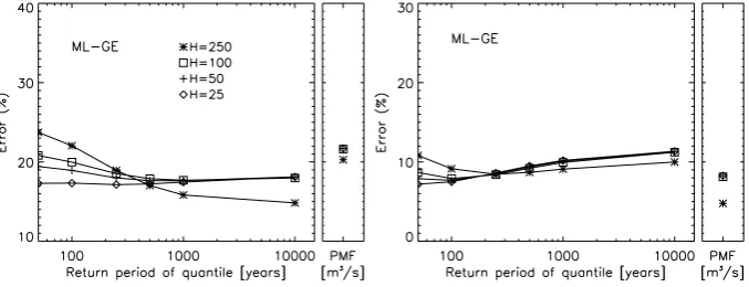
Fig. 5. Estimation error (in %) ofqˆT andgˆ(PMF estimate) for differentH.M=400 andN=50 years. Left: scenario 1, right: scenario 2.

with a return period equal toH. After this point, the estima-tion error is slightly higher, but remains in a similar order. It means that the Non-Systematic information contributes to re-duce the error in the flood quantiles estimation only for those quantiles of equal or larger return period than the threshold of perception.

6 Robustness analysis

Robustness analysis has been also made by Monte Carlo sim-ulations. Series have been generated coming from 3 different populations: (1) EV4 population, to analyse the robustness with respect to the selected upper bounded distribution in the case study; (2) TCEV population, in order to analyse robust-ness with respect to an unbounded distribution with 4 pa-rameters, which have shown good results in Mediterranean rivers; and (3) GEV population, to analyse robustness with respect to an unbounded distribution commonly used when dealing with flood frequency analysis. In this section, we will assume “similar error” if the estimation error increment is smaller than 50%. The estimation method was ML-GE for the EV4 and ML for the TCEV and GEV.

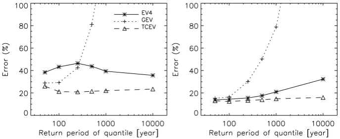
When an EV4 population is assumed (Fig. 6), or in other words, if the flood population has an upper bound, the quan-tiles estimated with EV4 and TCEV distributions give similar

errors in scenario 1, at least up to the estimation of 10 000 years return period quantiles, whereas for scenario 2 (lower skewness coefficient), the TCEV can be used with confidence below 1000 years. On the other hand, the GEVqˆT error is larger than 80% forT >200 years in both scenarios.

Fig. 6. Estimation error (in %) ofqˆT for EV4, GEV and TCEV distribution functions, assuming an EV4 population.H=50,M=400 and

N=50 years. Left: scenario 1, right: scenario 2.

Fig. 7. Estimation error (in %) ofqˆT for EV4, GEV and TCEV distribution functions, assuming a GEV population. H=50,M=400 and

N=50 years. Left: scenario 1, right: scenario 2.

Fig. 8. Estimation error (in %) ofqˆT for EV4, GEV and TCEV distribution functions, assuming a TCEV population.H=50,M=400 and

N=50 years. Left: scenario 1, right: scenario 2.

If TCEV and EV4 behaviours are compared, it should be underlined how similar they are from robustness point of view: both distributions have a limited estimation error in-crement for high skewness coefficient (scenario 1, Figs. 6 and 8 left) and increasing with return period for relative low skewness coefficient (scenario 2, Figs. 6 and 8 right). If we

7 Conclusions

Dealing with PMP or PMF, a general assumption in the hydrological community is that these upper bounds can be only estimated deterministically, with the single exception of El´ıasson (1994) for PMP estimation. However, it has been rigorously shown in this paper that, using statistical analysis with upper bounded distribution functions and introducing additional Non-Systematic information, it is possible to es-timate very high return period quantiles and the PMF with acceptable and similar estimation errors, as it is shown in Figs. 4 and 5.

Based on the ML method, three different methodologies to estimate the parameters of the bounded distribution functions can be implemented, depending on the available flood infor-mation. If there is a good deterministic a priori estimation of the PMF, the ML-GP method is advised. Otherwise, ML-C can be used considering the upper limit as one more param-eter. But in some combinations of distribution function and information (for example, the EV4 and TDF with additional CE Non-Systematic information), the upper limit estimated by ML-C method is equal to the maximum observation. In these situations, only the ML-GE method can be used.

Between the LN4, TDF and EV4 upper bounded distribu-tion funcdistribu-tions, the latest is the distribudistribu-tion funcdistribu-tion which better represents the shape of the empirical distribution func-tion of the Jucar River, which has a high skewness coefficient and, consequently, in accordance with the results obtained by Takara and Loebis (1996) and Takara and Tosa (1999). Com-bining this distribution function with the three proposed pa-rameter estimation methods, the Jucar series has been fitted and it has been possible to estimate statistically a PMF value for this river with an error of 50% (obtained by Monte Carlo analysis). In any case, the resulting estimate is not out the possible range of the Jucar River PMF at its sea mouth.

The uncertainty analysis shows that the EV4/ML-GE sta-tistical model is the most adequate among those presented in this paper, for the estimation of high return period quan-tiles and PMF when dealing with CE type Non-Systematic information.

For the sensitivity analysis case study (with more histor-ical information than in the Jucar River), the qˆ10 000 and

ˆ

g (PMF estimate) estimation error using the EV4/ML-GE model is approximately about 20%. Nevertheless, this model shows a slight sensitivity to the sample skewness, giving a reduction for theqˆT andgˆestimation error as the skewness coefficient is reduced. It must be pointed out thegˆerror with all methods is close to theqˆ10 000 error. Actually, if we ac-knowledge the 10 000 years return period quantile estimation error is admissible, we must admit also thegˆestimation error using the statistical approach given by ML-C or ML-GE.

Theqˆ10 000error obtained with the model EV4/ML-PG is approximately the error associated with the deterministic es-timation of the PMF. It means that if it is available a previ-ous value of the PMF, with its associated uncertainty, it is

possible to estimate high return period quantiles with equal or less uncertainty using the EV4/ML-PG model. However, introducing a prior estimation ofGwith relative small errors (as we are using in this work) is worst than do not use it and estimate it statistically by ML-GE or ML-C methods (Fig. 4). For the information scenario used in the robustness analy-sis, it can be concluded the EV4/ML-GE model can satisfac-tory fit samples coming from unbounded populations (GEV, Fig. 7) or unbounded mixed populations (TCEV, Fig. 8). On the contrary, if the flood population is upper bounded, the TCEV distribution function in general cannot be used for very high return periods and the GEV distribution function only can be accepted for the estimation of low return pe-riod quantiles, as it is shown in Fig. 6. So, it can be gen-eralized with an upper bounded population, the quantiles estimated using unbounded distributions with return period large enough, will be higher than the PMF and, consequently, with large unacceptable errors. For return periods producing quantiles similar to or smaller than the PMF, the error incre-ment compared with the use of the “true” upper bounded dis-tribution will depend of the fitted right tail disdis-tribution prop-erties.

Acknowledgements. This research was funded by the European

project SPHERE (EVG1-CT-1999-00010), a doctoral scholarship of the Universidad Polit´ecnica de Valencia and the Spanish project FLOODMED (CGL2008-06474-C02-02/BTE). Also we are very grateful to the comments of Dr. A. Kijko, Director of the Benfield Natural Hazard Centre at University of Pretoria, who gave us bright ideas in the precise moment of our research work.

Edited by: F. Laio

References

American Society of Civil Engineers (ASCE): Evaluation proce-dures for hydrologic safety of dams, Spillway Design Flood Selection, Surface Water Hydrology Committee, Report 8726– 26520, ASCE, New York, USA, 1988.

Benito, G., Lang, M., Barriendos, M., Llasat, M. C., Frances, F., Ouarda, T., Thorndycraft, V. R., Enzel, Y., Bardossy, A., Coeur, D., and Bob´ee, B.: Use of Systematic, Palaeoflood and Historical Data for the improvement of flood risk estimation, Review of scientific methods, Nat. Hazards, 31, 623–643, 2004.

Botero, B. A.: Estimaci´on de Crecidas de alto per´ıodo de retorno mediante funciones de distribuci´on con l´ımite superior e infor-maci´on No Sistem´atica, Ph.D. dissertation, Department of Hy-draulic Engineering and Environment, Polytechnic University of Valencia, 223 pp., 2006.

Calenda, G., Mancini, C. P., and Volpi, E.: Distribution of the ex-treme peak floods of the Tiber River from the XV century, Adv. Water Resour., 28(5), 615–625, 2005.

Cifres, E. and Abad, P.: Assessing the PMF for its use in the Algar Dam Project, in: Proceedings of the International Symposium on Dams and Extreme Floods, ICOLD–CIGB, Granada, Spain, 16 September 1992, 91–100, 1992.

Cohn, T. A. and Stedinger, J. R.: Use of Historical Information in a Maximum-Likelihood Framework, J. Hydrol., 96, 215–223, 1987.

Cohn, T. A., Lane, W. L., and Baier, W. G.: An Algorithm for Com-puting Moment-Based Flood Quantile Estimates when Historical Flood Information is available, Water Resour. Res., 33(8), 2089– 2096, 1997.

Condie, R. and Lee, K. A.: Flood Frequency Analysis with Historic Information, J. Hydrol., 58, 47–61. 1982.

Cooke, P.: Statistical Inference for Bounds of Random Variables, Biometrika, 66, 367–374, 1979.

Cunnane, C.: Review of Statistical Models for Flood Frequency Estimation, in: Hydrologic frequency modelling: Proceedings of the International Symposium on Flood Frequency and Risk Analysis, Baton Rouge, USA, 14–17 May 1986, 49–96, 1986. El´ıasson, J.: Statistical Estimates of PMP Values, Nord. Hydrol.,

25, 301–312, 1994.

El´ıasson, J.: A Statistical Model for Extreme Precipitation, Water Resour. Res., 33(3), 449–455, 1997.

England, J. F., Jarrett, R. D., and Salas, J. D.: Data-Based Compar-isons of Moments Estimators Using Historical and Paleoflood Data, J. Hydrol., 278, 172–196, 2003.

Enzel, Y., Ely, L. L., House, P. K., Baker, V. R., and Webb, R. H.: Paleoflood Evidence for Natural Upper Bound to Flood Magni-tudes in the Colorado River Basin, Water Resour. Res., 29(6), 2287–2297, 1993.

Frances, F.: Using the TCEV Distribution Function with Systematic and Non-Systematic Data in a Regional Flood Frequency Anal-ysis, Stoch. Hydrol. Hydraul., 12, 267–283, 1998.

Frances, F., Salas, J. D. and Boes, D. C.: Flood Frequency Analysis with Systematic and Historical or Paleofood Data Based on the Two Parameter General Extreme Value Models, Water Resour. Res., 30(5), 1653–1664, 1994.

Guo, S. L. and Cunnane, C.: Evaluation of the Usefulness of Histor-ical and PalaeologHistor-ical Floods in Quantile Estimation, J. Hydrol., 129, 245–262, 1991.

Hirsch, R. M. and Stedinger, J. R.: Plotting Positions for Historical Floods and Their Precision, Water Resour. Res., 23(4), 715–727, 1987.

Hosking, J. R. M. and Wallis, J. R.: Paleofood Hydrology and Flood Frequency Analysis, Water Resour. Res., 22(4), 543–550, 1986. Jarrett, R. D. and Tomlinson, E. M.: Regional Interdisciplinary

Pa-leoflood Approach to Assess Extreme Flood Potential, Water Re-sour. Res., 36(9), 2957–2984, 2000.

Jin, M. and Stedinger, J. R.: Flood Frequency Analysis with Re-gional and Historical Information, Water Resour. Res., 25(4), 925–936, 1989.

Kanda, J.: A New Value Distribution with lower and upper Limits for earthquake motions and wind speeds, Theor. Appl. Mech., 31, 351–360, 1981.

Kijko, A.: Estimation of the Maximum Earthquake Magnitude-Mmax, Pure Appl. Geophys., 161, 1–27, 2004.

Kijko, A. and Sellevoll, M. A.: Estimation of earthquake hazard pa-rameters form incomplete data files, part I, Utilization of extreme and complete catalogues with different threshold magnitudes, B.

Seismolog. Soc. Am., 79, 645–654, 1989.

Klemeˇs, V.: Probability of extreme hydrometeorological events: A different approach, in: Extreme Hydrological Events: Precipita-tion, Floods and Droughts, edited by: Kundzewicz, Z. W., Rosb-jerg, D., Simonovic, S. P., and Takeuchi, K., IAHS-AISH P., 213, 167–176, 1993.

Kroll, C. and Stedinger, J. R.: Estimation of Moments and Quantiles Using Censored Data, Water Resour. Res., 32(4) 1005–1012, 1996.

Lang, M., Ouarda, T. B. M. J., and Bob´ee, B.: Towards Operational Guidelines for Over-Threshold Modelling, J. Hydrol., 225, 103– 117, 1999.

Lang, M., Renard, B., Dindar, L., Lemaitre, F., and Bois, P.: Use of Statistical Test Based on Poisson Process for Detection of Changes in Peak-Over-Threshold Series, in: Hydrology: Science Practice for the 21st Century, Proceedings of the London Confer-ence, London, UK, 12–16 July 2004, 1, 158–164, 2004. Leese, M.: Use of Censored Data in the Estimation of Gumbel

Dis-tribution Parameters for Annual Maximum Flood Series, Water Resour. Res., 9(5), 1534–1542, 1973.

Martins, E. S. and Stedinger, J. R.: Historical Information in Gen-eralized Maximum Likelihood Framework with Partial Duration and Annual Maximum Series, Water Resour. Res., 37(9), 2559– 2567, 2001.

Merz, R. and Bl¨oschl, G.: Flood frequency hydrology: 1. Temporal, spatial, and causal expansion of information, Water Resour. Res., 44, W08432, doi:10.1029/2007WR006744, 2008.

Naghettini, M., Potter, K. W., and Illangasekare, T.: Estimating the upper tail of flood-peak frequency distributions using hydrome-teorological information, Water Resour. Res., 32(5), 1729–1740, 1996.

Naulet, R.: Utilisation de L’ information Des Crues Historiques Pour Une Meilleure Pr´ed´etermination Du Risque D’ inonda-tion, Ph.D. dissertainonda-tion, Universit´e Joseph Fourier, Universit´e du Qu´ebec Institut national de la recherche scientifique, France, 133 pp., 2002.

Naulet, R., Lang, M., Ouarda, T. B. M. J., Coeur, D., Bobee, B., Recking, A., and Moussay, D.: Flood Frequency Analysis on the Ardeche River Using French Documentary Sources from the Last Two Centuries, J. Hydrol., 313, 58–78, 2005.

O’Connell, D. R. H., Ostenaa, D. A., Levish, D. R., and Klinger, R. E.: Bayesian Flood Frequency Analysis with Paleohydrologic Bound Data, Water Resour. Res., 38(4), 16.1–16.13, 2002. Phien, H. N. and Fang T. E.: Maximum Likelihood Estimation

of the Parameters and Quantiles of the General Extreme-Value Distribution from Censored Samples, J. Hydrol., 105, 139–155, 1989.

Pilon, P. J. and Adamowski, K.: Asymptotic Variance of Flood Quantile in Log Pearson Type III Distribution with Historical In-formation, J. Hydrol., 143, 481–503, 1993.

Reis, D. S. and Stedinger, J. R.: Bayesian MCMC Flood Frequency Analysis with Historical Information, J. Hydrol., 313, 97–116, 2005.

Rigo, T. and Llasat, M. C.: Analysis of mesoscale convective systems in Catalonia using meteorological radar for the period 1996–2000, Atmos. Res., 83, 458–472, 2007.

Slade, J.: An Asymmetric Probability Function, T. Am. Soc. Civil Eng., 62, 35–104, 1936.

Smith, K. and Ward, R.: Floods. Physical Processes and Human Impacts, John Wiley and Sons, Baffins Lane, Chichester, UK, 1998.

Stedinger, J. R. and Cohn, T. A.: Flood Frequency Analysis with Historical and Paleoflood Information, Water Resour. Res., 22(8), 785–793, 1986.

Stedinger, J. R. and Baker, V. R.: Surface Water Hydrology: Histor-ical and Paleofood Information, Rev. Geophys., 252, 119–124, 1987.

Stevens, E. W.: Uncertainty of Extreme Flood Estimates Incorporat-ing Historical Data, Water Resour. Bull., 286, 1057–1068, 1992.

Takara, K. and Loebis, J.: Frequency Analysis Introducing Proba-ble Maximum Hydrologic Events: Preliminary Studies in Japan and in Indonesia, in: Proceedings of International Symposium on Comparative Research on Hydrology and Water Resources in Southeast Asia and the Pacific, Yogyakarta, Indonesia, 18– 22 November 1996, Indonesian National Committee for Interna-tional Hydrology Programme, 67–76, 1996.

Takara, K. and Tosa, K.: Storm and Flood Frequency Analysis Us-ing PMP/PMF Estimates, in: ProceedUs-ings of International Sym-posium on Floods and Droughts, Nanjing, China, 18–20 Octo-ber 1999, 7–17, 1999.

Williams, A. and Archer, D.: The use of historical flood information in the English Midlands to improve risk assessment, Hydrolog. Sci. J., 47(1), 57–76, 2002.