A two parameter design storm for Mediterranean convective rainfall

www.hydrol-earth-syst-sci.net/21/2377/2017/ doi:10.5194/hess-21-2377-2017

© Author(s) 2017. CC Attribution 3.0 License.

A two-parameter design storm for Mediterranean

convective rainfall

Rafael García-Bartual and Ignacio Andrés-Doménech

Universitat Politècnica de València, Instituto Universitario de Investigación de Ingeniería del Agua y Medio Ambiente (IIAMA), Camí de Vera s/n, 46022 Valencia, Spain

Correspondence to:Ignacio Andrés-Doménech ([email protected]) Received: 2 December 2016 – Discussion started: 12 December 2016 Revised: 28 March 2017 – Accepted: 15 April 2017 – Published: 9 May 2017

Abstract. The following research explores the feasibility of building effective design storms for extreme hydrologi-cal regimes, such as the one which characterizes the rain-fall regime of the east and south-east of the Iberian Penin-sula, without employing intensity–duration–frequency (IDF) curves as a starting point. Nowadays, after decades of func-tioning hydrological automatic networks, there is an abun-dance of high-resolution rainfall data with a reasonable statistic representation, which enable the direct research of temporal patterns and inner structures of rainfall events at a given geographic location, with the aim of establishing a sta-tistical synthesis directly based on those observed patterns. The authors propose a temporal design storm defined in ana-lytical terms, through a two-parameter gamma-type function. The two parameters are directly estimated from 73 indepen-dent storms iindepen-dentified from rainfall records of high tempo-ral resolution in Valencia (Spain). All the relevant analytical properties derived from that function are developed in order to use this storm in real applications. In particular, in order to assign a probability to the design storm (return period), an auxiliary variable combining maximum intensity and to-tal cumulated rainfall is introduced. As a result, for a given return period, a set of three storms with different duration, depth and peak intensity are defined. The consistency of the results is verified by means of comparison with the classic method of alternating blocks based on an IDF curve, for the above mentioned study case.

1 Introduction

Design storms are of paramount importance for hydrologic engineering and remain mainstream practice as they provide a simple and apparently appropriate tool for the design of hydraulic infrastructure. Design storms have been used for more than a century if we consider the block rainfall as input of the rational method (Watt and Marsalek, 2013). They ex-perienced an important development during the 1970s and 1980s with more realistic approaches being implemented (Pilgrim and Cordery, 1975; Walesh et al., 1979; Hogg, 1980, 1982; Pilgrim, 1987).

The need for design storms in hydrologic engineering must be analysed according to the spatial scale of the problem, which might range from typical urban drainage designs to small and intermediate catchment basins. As reported by Watt and Marsalek (2013), one of the earliest applications of design storms to urban drainage took place in Rochester, New York (Kuichling, 1889). It followed the rational method which is still widely used today. In the urban context, the City of Los Angeles method (Hicks, 1944) and the Chicago Hydrograph Method (Keifer and Chu, 1957) represented an important step towards the development of hydrograph meth-ods. On the watershed scale, design storms are needed to ob-tain design floods when streamflow data are scarce or do not exist (Watt and Marsalek, 2013) for the design of culverts, bridges and small dams, drainage systems, drainage plan-ning, and flood management.

Within the first category, the most widely used synthetic storms are probably the National Resource Conservation Ser-vice (NRCS, formerly SCS) dimensionless storms and the so-called alternating-block method storms. Standard rainfall patterns for 24 h storms are available for four different geo-graphic regions of the United States (Froehlich, 2009). The NRCS design storms are appropriate for catchments smaller than 250 km2, and they are considered to be applicable to storms of any average return period. Temporal distributions within this method are based on depth–duration–frequency relations available for the US territory, divided into four dif-ferent climatic regions (McCuen, 1989).

The alternating-block method (Chow et al., 1988) is solely based on an IDF curve. These design storms display a maxi-mum intensity block in the centre of the event and a total rain-fall depth at any time that coincides with the total depth given by the IDF relation. The method is simple but has also been widely criticized, because it does not represent any observed rainfall internal structure. Another noticeable weak point of the method, already pointed out by McPherson (1978), is the arbitrary selection of the storm duration, which causes to-tal rainfall depth to also be arbitrarily selected. The Chicago design storm (Keifer and Chu, 1957) is a special case of an alternating-block storm. In Spain, the use of this method is still today concretized through local or regional IDF curves such as those proposed by Témez for all the Iberian Peninsula (Témez, 1978). Recent publications demonstrate that, gener-ally, peak-flow calculations using these design storms tend to overestimate the results (Alfieri et al., 2008).

The second category of design storms corresponds to tem-poral patterns derived from observed records. One of the first temporal distributions using this approach was devel-oped by Huff (1967) in Illinois (US). The method determines in which time quartile the maximum intensity occurs. This work eventually became the Illinois State Water Survey De-sign Storm (Huff and Angel, 1989), extensively used by state and local agencies in the US Midwest. Following the same methodology, Hogg (1980) presented his findings on tempo-ral patterns depending on the storm duration for different re-gions in Canada. Results led to the AES design storm (Hogg, 1982), widely used in urban drainage design. The former de-sign storm reproduces the maximum intensity, the time of this maximum and the rainfall depth that occurs before the peak on the basis of observed records. Other works into this category are those developed in Australia (Pilgrim, 1987; French and Jones, 2012) or the UK (Packman and Kidd, 1980). In Spain, García-Bartual and Marco (1990) studied hyetographs of extreme convective precipitation where the intensity resulting from the activity of each rainfall cell was represented by a gamma-type function with maximum inten-sity and volume as random variables.

Some authors point out that the design storm concept it-self is fraught with conceptual error when used to simplify engineer analysis with unrealistic assumptions (Adams and Howard, 1986). Indeed, many of the concerns about

clas-sic design storms arise from the storm duration selection, the IDF concept limitations, the temporal distribution and the difficulties of relating the synthetic storm event to a specific return period.

The design storm duration is not a determining factor if the purpose is to determine a peak flow to design conveyance infrastructures. Consequently, it is common practice to fix it around the concentration time of the catchment basin. Never-theless, when storage elements are to be analysed, the influ-ence of storm duration and temporal pattern becomes critical (Ball, 1994).

As has been shown in the past (Watt and Marsalek, 2013), uncertainties arising from existing IDF relations have strong consequences. First, record series used to fit IDF expres-sions are usually short for low-frequency occurrences. Sec-ond, IDF curves are considered to represent worst maxima regardless of the physical nature of the storm. García-Bartual and Schneider (2001) exposed the inherent uncertainty in the process, which significantly affects the definition of the IDF curves’ shape in the interval 0–10 min. Finally, there is enough reason to deem data acquisition insufficiently accu-rate in providing robust data for IDF analysis, especially in urban areas (Hoppe, 2008). Moreover, as is the case in Spain, outdated IDF curves are still regularly used, as they are still found in guidance and regulations. The above mentioned un-certainties in IDF curves’ estimation can significantly affect the reliability of derived design storms, especially in the def-inition of its peak rainfall intensities, with undesirable con-sequences when used for hydrologic design purposes.

For the simplest applications (i.e. rational method), a tem-poral pattern is not required for the design storm. However, for most hydrologic engineering applications, a design hyeto-graph is necessary. Selecting this temporal trend is one of the most uncertain steps of the design storm definition, since the physical nature of the process cannot be disregarded.

A storm event presents many characteristics, so it cannot be fully described by the statistics of only one of them. For a return period definition, a common practice is to assign a given frequency to a specific event feature (i.e. its maximum intensity). But, given that a design storm is composed of many variables (depth, duration, temporal pattern, antecedent conditions), assigning a single return period may not be ap-propriate.

2 Design storm

The temporal pattern of rainfall intensities representing the design storm is expressed in terms of a continuous analytical function of the form given as follows:

i (t )=i0f (t ), (1)

where t ≥0 (min) is the time elapsed from the start of the rainfall episode (t=0), i(t ) (mm h−1) represents the rain-fall intensity at instant t,i0 (mm h−1) is the instantaneous

peak intensity of the storm and f (t ) is a convenient non-dimensional, continuous and differentiable analytical func-tion, which will be defined below.

The adopted functionf (t )must reproduce the activity life cycle of a convective cell, i.e. an initial development until the maturity stage is reached, during which maximum intensi-ties are attained, followed by a stage of dissipation in time, typified by a progressive attenuation of rainfall.

Several recent studies characterize the physical dynam-ics of convective cells from radar-provided data. More pre-cisely, these data correspond to relevant characteristics such as duration, spatial extension or the importance of the above-mentioned stages, (Capsoni et al., 2009; Rigo and Llasat, 2005). On the basis of high-resolution rainfall data, some au-thors report statistical evidence of the predominance of tem-poral patterns where the attenuation or temtem-poral dissipation stages tend to last longer than the initial growing and de-velopment stage (Brummer, 1984). This characteristic sup-ports the use of relationships like the gamma function, suc-cessfully employed in previous mathematical models of rain-fall (García-Bartual and Marco, 1990; Salsón and Garcia-Bartual, 2003) since it represents more accurately the pat-terns observed in the temporal registers of convective rainfall events in the east and south-east of the Iberian Peninsula. Nonetheless, there are other mathematical models where an analytic functionf (t )is postulated, and where the maximum value is located precisely at half the total duration of the event produced by the convective cell (Northrop and Stone, 2005).

In terms of the proposed design storm, the adopted tem-poral pattern shows an evolution described in a parametrical way with a function f (t ): a non-dimensional gamma-type function with a single parameter which describes a fast ini-tial growing stage of intensities until reaching the maximum value, followed by a slower diminishing stage, asymptotic in time and tending towards a null value when time is growing towards infinity.

f (t )=ϕt e1−ϕt, (2)

whereϕ(min−1)is a parameter.

This model proved to be an acceptable and consistent representation of the rainfall intensities from convective Mediterranean storms (Andrés-Doménech et al., 2016)

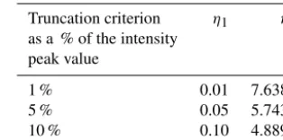
Table 1.Parametersη1andη2for different truncation criteria.

Truncation criterion η1 η2

as a % of the intensity peak value

1 % 0.01 7.6386

5 % 0.05 5.7439

10 % 0.10 4.8897

2.1 Analytical properties

Some interesting analytical properties of the f (t )function are revised, which will prove useful in subsequent develop-ment. The following can be deduced from Eq. (2):

f (0)=0, (3)

lim

t→∞f (t )=0. (4)

In addition, as

f0(t )=ϕ (1−ϕt ) e1−ϕt, (5)

functionf (t )displays a relative maximum at pointt=t0=

ϕ−1. The corresponding value of this maximum is as follows:

f (t0)=1. (6)

Given that the duration,tC, of the cell is finite, and in order to

establish a finite duration of the process, a simple truncating criteria is adopted for the asymptote of this function. To do so, a final or residual value is established as a fractionη1of

the maximum so that

f (tC)=η1, (7)

where tC (min) represents the total storm duration, with

tC>t0and 0 <η1< 1. Convenientη1values are shown in

Ta-ble 1. Introducing conditions given in Eq. (7) into Eq. (2), we obtain the following:

f (tC)=ϕtCe1−ϕtC=η1. (8)

Equation (8) admits the following solution:

tC=

η2

ϕ, (9)

and thus verifies the condition

η2e1−η2 =η1. (10)

Table 1 shows some of the solution values for this equation, for chosen values of the parameterη1.

2.2 Properties of the aggregated process

The suggested analytical function can be integrated, yielding to the following result:

F[t1;t2]= Z t2

t1

f (t )dt=

Z t2

t1

ϕt e1−ϕtdt=

t1+

1

ϕ

e1−ϕt1

−

t2+

1

ϕ

e1−ϕt2_{, (11)}

where 0≤t1<t2≤tC. In this way, the integrated value of

F[t1;t2] is expressed in minutes. By applying Eqs. (9) and

(11), the following particular results are easily obtained:

F[0;tC]= e ϕ−

tC+

1

ϕ

e1−ϕtC₌ e ϕ

1−(1+η2) e−η2

, (12)

F[0;∞]=

e

ϕ, (13)

F[0;tC] F[0;∞]

=1−(1+η2) e−η2. (14)

It must be noted that the result of Eq. (14) is independent of parameterϕ. For instance, if a truncating value of 5 % is adopted (η1=0.05), it automatically leads toη2=5.7439 as

shown in Table 1, and therefore

F[0;tC] F[0;∞]

=0.98. (15)

That is, the truncating criteria of 5 % for f (t )is equivalent to establishing the total duration of the cell when 98 % of the cumulative rainfall has already taken place with respect to the hypothetical 100 % linked to a cell whose intensities are asymptotic to 0 and have infinite duration, according to the known analytical properties of the tail off (t ).

From Eqs. (1) and (11), the total cumulative rainfall (mm) can be obtained, for a given time interval, [t1;t2], as follows:

P[t1;t2]= Z t2

t1

i (t )dt= i0

60 Z t2

t1 f (t )dt

= i0

60

t1+

1

ϕ

e1−ϕt1₋

t2+

1

ϕ

e1−ϕt2

. (16)

The average rainfall intensity (mm h−1) during such a given time interval can be calculated as follows:

i[t1;t2]= i0

t2−t1

t1+

1

ϕ

e1−ϕt1₋

t2+

1

ϕ

e1−ϕt2

.

(17) In the same manner, the total cumulative rainfall for the time interval [0;t] results in the following:

P[0;t]=

i0 60 _e ϕ − t+1

ϕ

e1−ϕt

. (18)

Replacingt=tCin Eq. (18) and substituting Eq. (9), we

ob-tain the total rainfall for the theoretical storm, given by the following expression:

P[0;tC]= i0 60 _e ϕ − _η 2 ϕ + 1 ϕ

e1−η2

. (19)

If we assume a truncating criteria of 5 % (η1=0.05) a

straightforward expression is obtained for the total cumula-tive rainfall associated with the analytical storm:

P[0;tC]=0.0443 i0

ϕ. (20)

2.3 Maximum intensity for a given1t

For practical applications, a given time interval of aggrega-tion1t is used, conveniently chosen depending on the type of hydrological application, the rainfall–runoff model to be used, and the characteristics of the urban hydrology applica-tion to be carried out.

Once a given1t(in minutes) is selected, it is convenient to locate the most intense rainfall interval along the time axes, so that

I1t=

i0

60max

F[t;t+1t] , (21)

wheret<t0<t+1t andI1t is the maximum rainfall inten-sity (mm h−1_{), for the most intense interval of the storm, as}

shown in Fig. 1.

If the above-mentioned central interval is [tL;tU]=

₁ ϕ−ξ 1t;

1

ϕ+(1−ξ ) 1t

, (22)

as indicated in Fig. 1, the optimization problem has a solution in terms of the auxiliary variableξ, being 0 <ξ< 1. Such a solution is given by the following:

ξ= 1 ϕ1t −

e−ϕ1t

1−e−ϕ1t. (23)

Consequently, according to Eq. (17), the maximum intensity of the storm, once it has been discretized in time intervals of

1tminutes, can be calculated as follows:

I1t=

i0

1t

tL+ 1

ϕ

e1−ϕtL₋

tU+

1

ϕ

e1−ϕtU

. (24)

In summary, the main derived properties of the chosen an-alytical shape of the storm are total duration of the storm given a truncation criterion (Eq. 9), total cumulative rainfall (Eq. 20) and maximum intensity for a given time level of aggregation1t(Eq. 24). All these relations are uniquely ex-pressed as functions of the two parameters of the storm,i0

i0

t0

tL tU

i(t)

₁i0

t tC

t

Figure 1.Most intense interval of the storm defined by [tL;tU] for

a1ttime interval of aggregation.

3 Rainfall data processing

Valencia is a Mediterranean city, located on the eastern coast of the Iberian Peninsula. It presents a typical temperate Mediterranean climate (Csa, according to Köppen climate classification). This type of climate is characterized by mild temperatures (annual average of 17◦C), without marked ex-tremes and with a rainfall of about 450 mm yr−1. Rainfall is very unevenly distributed throughout the year, with very marked minima during the months of June, July and August and maxima happening during the months of September and October, these two months concentrating almost a third of the annual rainfall.

Another important characteristic of the rainfall regime is its irregularity, alternating dry and more humid intervals. These dry or humid periods tend to last several years due to the Mediterranean climatic inertia. The torrential character of storms is also a main feature of the rainfall regime of the region, with frequent convective rainfall mesoscale episodes, most widely known as cut-offs, characterized by very local-ized high-intensity storms.

The rainfall series used in this study were recorded by the Júcar River Basin Authority during the period 1990–2012. The rainfall gauge is installed in the city centre and the data time step is 5 min. Previous studies demonstrated the validity of this data set for similar purposes (Andrés-Doménech et al., 2010). The continuous rainfall series are processed to iden-tify and extract convective storms. First, statistically indepen-dent rainfall events are iindepen-dentified. Then, amongst them, only convective events are extracted. Finally, convective storms are identified from convective events and finally selected to estimate model parameters.

3.1 Convective storms set

3.1.1 Identification of statistically independent rainfall episodes

Before undertaking the storm analysis, a preliminary step is required in order to separate the original continuous se-ries of rainfall records in statistically independent rainfall events. There is no universal method for identifying the min-imum inter-event time of a rainfall regime and, thus, inde-pendent storms. Dunkerley (2008) presents an interesting re-view of the range of approaches used in the recognition of main events. Early works by Restrepo-Posada and Eagle-son (1982) are still in force, and according to them the identi-fication of independent events is based on considering events such as statistically independent events, so that the minimum inter-event time must be an outcome of a Poisson process. Bonta and Rao (1988) bore out this theory, studying some other aspects in depth. Andrés-Doménech et al. (2010) com-pleted the original methodology based on the coefficient of variation analysis and established for Valencia a minimum inter-event time equal to 22 h. The latter implies that if two rainfall pulses are separated by more than 22 h, then, they be-long to different events. Under this premise, 987 statistically independent events are identified for the period 1990–2012. 3.1.2 Identification of convective episodes

The required rainfall episodes must have a certain convec-tive character. Therefore, only storms that verify the follow-ing conditions can be taken into account: maximum intensity over 35 mm h−1 and convectivity index β∗> 0.3. The con-vectivity index introduced by Llasat (2001) reflects in an objective way the greater or lesser convectivity degree of a rainfall episode, on the sole basis of the registered 5 min data, with no additional meteorological information being required. The valueβ∗depends on a convectivity threshold which depends itself on the record time step. This convec-tivity threshold was estimated for the Spanish Mediterranean coastline by Llasat (2001). For a 5 min resolution data series, the threshold was set to 35 mm h−1. Consequently, this in-dex represents the proportion of total rainfall fallen with an intensity higher than 35 mm h−1. Events with β∗> 0.3 rep-resent convective storms at this location. Thus, according to this additional criterion, only 64 convective events from the complete set are selected.

3.1.3 Selection of convective storms

Some of the independent convective events selected above can correspond to long or very long episodes with important dry intra-periods (always less than 22 h). Concatenation of some convective cells can lead to this situation, resulting in long episodes on some days.

these convective cells only correspond to a small duration within the whole episode. Nevertheless, they can represent more than 80 % of the total rainfall amount. According to this fact, the convective events set is classified as follows.

a. Type I events: these storms consist of a single convec-tive cell. They are characterized by a moderate duration and a considerable average intensity. They can present low-intensity intervals before and/or after the larger part of rainfall.

b. Type II events: long-lasting rainfall events consisting of two or more storms separated in time.

Following this classification, 58 events are type I and 6 events are type II. These 6 type II events are carefully examined and analysed to extract storms within them. The following criteria to select individual storms are adopted:

a. Identify the event peak intensity, always over 35 mm h−1, and its near range.

b. The first storm time interval corresponds to the prior in-terval to 9.6 mm h−1 intensity (3 times the rain gauge sensitivity).

c. The last storm time interval is defined by a shift in the sign of the hyetograph derivative, always around inten-sities lower than 9.6 mm h−1.

Finally, and according to this methodology, 73 storms are de-fined for the period 1990–2012. Table 2 shows a basic report of the empirical statistics of this sample. Andrés-Doménech et al. (2016) also pointed out a strong correlation between the storm volume and duration (0.839) and also an evident cor-relation between storm volume and its maximum intensity (0.639).

3.2 Relations between cumulative rainfall and maximum intensity of the storm

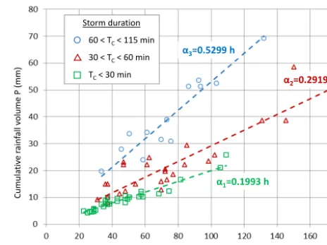
Three different sets of events were identified, according to their duration. As shown in Fig. 2, each of them can be char-acterized in terms of a representative value of the following ratio.

αi=

P I10

(25) Figure 2 shows the three different ratios empirically found:

α1=0.1993 h,α2=0.2919 h andα3=0.5299 h.

Such distinction allows for the identification of three dif-ferent families, depending onαi. Each of them is character-ized by its corresponding storm pattern. In accordance with this, a given return periodT should yield to three storms, one per family, all of them with equivalent magnitude, but with different time patterns. Low α values typically correspond with storms with peak intensity occurring shortly after the initiation of the storm, while higherα values are found for longer events and usually higher cumulative rainfall depths.

α1=0.1993 h

α2=0.2919 h α3=0.5299 h

Storm duration

60 < TC< 115 min

30 < TC< 60 min

TC< 30 min

Cumula

tiv

e

ra

in

fa

ll

vo

lume

P

 (mm)

Maximumintensitywitha 10‐min aggregationlevelI10 (mmh–1)

Figure 2.Relations between cumulative rainfall and maximum in-tensity of the storm depending on the storm duration.

3.3 Storm magnitude

The question of determining the magnitude of a given storm is undertaken through a principal-component analysis (PCA), over the observed sample (I10;P). This strategy is

based on the fact that both maximum intensity and cumu-lative rainfall are directly related to the magnitude of the event, and are thus relevant to it, while the preliminary sta-tistical analysis showed a significant correlation among them as stated before (Andrés-Doménech et al., 2016).

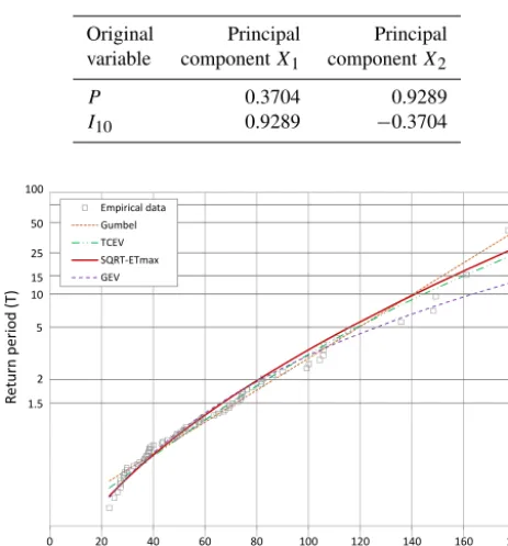
Table 3 shows the results of the principal-component anal-ysis, resulting in the two new variables,X1andX2.

It can be noted that the first main component,X1, explains

92.1 % of the variance observed in the sample. This main component is defined as

X1=βPP+βII10=0.3704P +0.9289I10. (26)

According to the relationships between the cumulative rain-fall depth and the storm maximum intensity, both variables are used together to define a new combined variable that is able to represent the storm magnitude in terms of volume and maximum intensity.X1can be considered a measurement of

the magnitude of the rainfall event, as both initial variables,

P andI10, contribute to it. This new variable after the PCA

analysis, in statistical terms, contains more information by itself than eitherP orI10, and thus represents an adequate

variable in order to establish a return period,T, linked to a given design storm.

3.4 Return period

The process of assigning a return periodT to a given de-sign storm should be based on a previous statistical anal-ysis of the selected variable, X1. To do so, an appropriate

Table 2.Storm univariate statistics (adapted from Andrés-Doménech et al., 2016).

Rainfall volume Maximum intensity Storm duration

P (mm) I10(mm h−1) TC(min)

Mean 20.0 76.4 38.0

Maximum 69.2 206.4 115.0

Minimum 4.2 36.0 10.0

Median 15.0 64.8 30.0

Standard deviation 15.9 37.3 21.9

Bias 1.39 1.46 1.21

Kurtosis 1.36 2.09 1.18

Table 3.Principal-component eigenvectors resulting from the PCA analysis.

Original Principal Principal

variable componentX1 componentX2

P 0.3704 0.9289

I10 0.9289 −0.3704

0 20 40 60 80 100 120 140 160 180

R

eturn period (T)

Principal component X1

Empirical data Gumbel TCEV SQRT‐ETmax GEV

2

1.5 5 15 25 50 100

10

Figure 3.Extreme value distribution analysis for principal

compo-nentX1.

tested, including Gumbel, two-component extreme value (TCEV), squared root exponential type distribution of max-imum (SQRT-ETmax) and general extreme value (GEV). In all cases, maximum likelihood was used to estimate the cor-responding parameters. Figure 3 shows the results of this ex-treme value function analysis. Best fit was obtained with the SQRT-ETmax distribution, with the advantage of being more parsimonious than TCEV and GEV functions. This result is in accordance with what usually occurs on the eastern coast-line of Spain.

4 Construction of the design storm

IfX1(T )is the quantile of the extreme value distribution

cor-responding to a given return periodT, the two variablesP

andI10, which define the design storm for that given return

period, are obtained by solving Eqs. (25) and (26) for each familyi=1, 2 and 3. That is,

  

 

I10,i(T )=

X1(T )

βI+βPαi

Pi(T )=

αiX1(T )

βI+βPαi

(27)

In order to define, in practice, the design storm associated withI10,i andPi values, and once chosen a convenient time level of aggregation (i.e.1t=10 min), it is necessary to ob-tain the two parameters,i0andϕ, which analytically define

the design storm. To do so, Eqs. (20) and (24) are used, and they result as follows, for eachi=1, 2 and 3:

Pi(T )=0.0443

i0,i

ϕi

, (28)

I10,i(T )=

i0

1t

tL+

1

ϕi

e1−ϕitL₋

tU+

1

ϕi

e1−ϕitU

,

(29) wheretL andtU are calculated according to Eqs. (22) and (23).

5 Comparison with the alternating-block design storm After formulating the practical steps to build a synthetic storm, a comparison of the former with the most widely used storm (built with alternating blocks obtained from an IDF curve), is performed. In order to carry out this comparison, storms corresponding to a return period of 25 years are built. The choice of 25 years corresponds to the requirements set by the Municipality of Valencia regulations for the design of urban drainage hydraulic infrastructures.

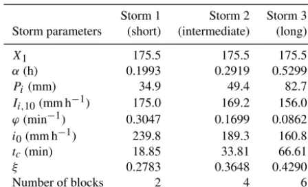
Table 4.Parameters for the three synthetic storms.

Storm 1 Storm 2 Storm 3

Storm parameters (short) (intermediate) (long)

X1 175.5 175.5 175.5

α(h) 0.1993 0.2919 0.5299

Pi(mm) 34.9 49.4 82.7

Ii,10(mm h−1) 175.0 169.2 156.0

ϕ(min−1) 0.3047 0.1699 0.0862

i0(mm h−1) 239.8 189.3 160.8

tc(min) 18.85 33.81 66.61

ξ 0.2783 0.3648 0.4290

Number of blocks 2 4 6

To do this, the usual procedure for obtaining IDF curves is followed, adjusting the empirical sample to the following IDF relation:

i(t )= a

(b+t )c, (30)

wherei (mm h−1) is the maximum intensity corresponding to a rainfall duration t (min), whilea,b andcare the pa-rameters of the IDF curve. Vaskova (2001) demonstrated the fitness of this expression for adjusting local IDF curves in Valencia. With the data employed in the present paper, the following coefficients result for the 25-year return period ID curve: a=8198 mm h−1,b=29.8 min andc=1.06. Then, for each case, the alternating-block design storm is built from the ID curve defined by Eq. (31), following the usual method-ology (Chow et al., 1988). To allow for a proper comparison with the Gamma storm, the same number of blocks is kept for every case.

To perform the comparison, first, the three synthetic storms corresponding to each of the families defined byα1

(short storms), α2 (medium duration storm) and α3 (long

storms) are built. In order to do this, once the truncating level has been setη1(0.05 in the present paper), the method

sum-marized in Sect. 4 is followed. For a return period of 25 years, it results in a storm magnitudeX1=175.5 (Fig. 3). A

con-tinuous storm for each of the three families is obtained and, after being discretized in blocks of 1t=10 min, generates, for each family, a storm of 2, 4 and 6 blocks respectively, as once the truncation criterion is selected, the storm dura-tion is established (Eq. 9), so that, for a given time level of aggregation (1T), the number of blocks can be derived. Ta-ble 4 summarizes the essential parameters of each of the three storms.

Figure 4 represents, for each family, both the contin-uous and the aggregated Gamma storms, along with the alternating-block storm obtained from the ID curve.

Both methods lead to consistent and relatively similar re-sults, those being particularly alike for the longer storms. However, for short- and medium-duration storms, it becomes clear that the classic method offers significantly more

pes-simistic results. In other words, the common method dis-plays higher intensities. This result is coherent with the well-known process of defining the storm. Indeed, given that the alternating-block method assumes the simultaneous occur-rence of maximum intensities for different durations, even when those values had not been encountered historically in the same rainfall event, overestimated intensities seem to be an unsurprising outcome. On the contrary, the Gamma storm is built directly from the temporal pattern observed in real episodes. That is, as demonstrated by Andrés-Doménech et al. (2016), the Gamma storm is coherent with the temporal structure of the rain process and that is why the proposed synthetic storm reproduces the observed rainfall more accu-rately. Table 5 gathers the quantitative differences found for each of the three storms.

As expected, the higher the duration of the storm, the lesser the difference between the maximum instant intensity of the continuous storm and the one of the maximum block. Furthermore, differences between the maximum block inten-sities between the aggregated Gamma storm and the alternat-ing block storm are also reduced as the duration of the storm increases.

Nonetheless, the most remarkable differences lie on rain-fall volumes. Given a return period, the alternating-block method combines in a single theoretical storm the most ad-verse statistics for several durations, which originally derive from different historical rainfall events. Conceptually, this is a worst-case-scenario storm ignoring actual rainfall patterns found in the rainfall registers, yielding to a volume overes-timation (Di Baldassarre et al., 2006). For the aggregated Gamma storm, differences with regard to the continuous model are more limited, in all cases, which supports the con-clusion of having generated a synthetic storm that not only reproduces peak intensities properly but also respects the ob-served temporal patterns and, consequently, reproduces bet-ter storm volumes. Concerning variable X1, results are very

similar for both methods, as shown in Table 5.

6 Conclusions

suffi-0 20 40 60 80 100 120 140 160 180 200 220 240

‐20 ‐10 0 10 20 30 40 50 60

Rai

nfal

l i

ntensi

ty (mm

h

–1)

Time (min)

Continuous Gamma model Aggregated Gamma model IDF alternating block model

0 20 40 60 80 100 120 140 160 180 200 220 240

‐20 ‐10 0 10 20 30 40 50 60

Rai

nfal

l i

ntensi

ty (mm

h

–1)

Time (min)

Continuous Gamma model Aggregated Gamma model IDF alternating  block model

0 20 40 60 80 100 120 140 160 180 200 220 240

‐20 ‐10 0 10 20 30 40 50 60

Rai

nfal

l i

ntensi

ty (mm

h

–1)

Time (min)

Continuous Gamma model Aggregated Gamma model IDF alternating block model

(a) (b) (c)

Figure 4. Comparison of the continuous and aggregated Gamma model with the IDF alternating-block model for the three families

α1=0.1993(a),α2=0.2919(b)andα3=0.5299(c)forT =25 years.

Table 5.Comparison of volume, peak intensity and magnitude of the Gamma-aggregated and IDF alternating-block design storms.

Duration Maximum intensity Volume Magnitude

(min) (mm h−1) (mm) X1

Stormα1 Gamma aggregated 20 175.0 34.8 175.45

IDF alternating block 20 164.4 43.2 168.71

Stormα2 Gamma aggregated 40 169.2 45.0 173.84

IDF alternating block 40 164.4 60.3 175.05

Stormα3 Gamma aggregated 60 156.0 80.9 174.87

IDF alternating block 60 164.4 69.3 178.38

ciently reliable or representative of the maximum rainfall of that location.

One of the downsides of this process is the fact that it ig-nores, in its approach, aspects relative to the actual duration and structure – or inner pattern – of intensities of rain, visible in high-resolution rainfall registers. In some countries, auto-matic pluviometer networks have been working for decades and thus, detailed information is now available, allowing en-gineers to undertake such matters with statistical representa-tivity (De Luca, 2014).

However, the diversity of hydraulic elements of current drainage systems (e.g. storm tanks, sustainable drainage sys-tems) means that most conditioning storm parameters for the design are not only rain intensities but also duration, total cumulated rainfall and temporal structure of the storm. This makes the exploration of new strategies for building design storms particularly interesting, starting directly from the ob-served patterns in the high-resolution registers, instead of us-ing IDF curves. This research explores the possibilities in this sense, for the case of convective-type Mediterranean storms and proposes a case study from the automatic pluviometer register of the city of Valencia.

The design storm is defined in an analytical way through a two-parameter function (i0 andϕ), already substantiated

by previous studies for the Mediterranean area. The former parameters are estimated directly from independent rainfall events, identified in the original temporal series. The assign-ment of a return period is done through an auxiliary vari-able which describes the magnitude of the event, and in-corporates simultaneously both the total cumulated rainfall and the maximum intensity. In practice, this criterion leads to three different design storms for each return period, of a similar magnitude but with different temporal patterns and durations. Those storms, exclusively defined in terms of the two pointed parameters, are easily discretized in time inter-vals1t, in view of their application to practical cases.

de-termination of the storm without using IDF curves. Naturally, it has the important limitation of being only applicable in ge-ographic locations where there is high-resolution rainfall in-formation of sufficient quality and appropriate length of his-torical record series. In the future, for a higher statistical rep-resentativity, it will become necessary to count with a longer register.

The proposed method herein, as well as other simple de-sign storm approaches, present some inherent limitations for certain hydrological engineering applications, as they are not suitable for case studies where a more detailed or compre-hensive description of the rainfall process is required. Some examples are continuous-time hydrological-system evalua-tion, hydrological applications in large catchments, or appli-cations where ensembles or stochastic generation of events are needed to account for a number of possible scenarios (Frances et al., 2012).

Despite that, the proposed analytical definition defines a feasible work framework to provide the design storm with the spatio-temporal dimension of the event, through the ad-dition of a component that considers the decline of intensities from the centre of the cell. By following the practical strategy contained in the present paper, the characterization and esti-mation of parameters of such a component must be founded on the direct observation of radar data for the most significant storms, with the goal of parametrizing the most characteristic spatial patterns (Barnolas et al., 2010).

Data availability. Detailed information on the storm data set can be accessed at https://riunet.upv.es/handle/10251/75033. Additional information regarding the data availability can be obtained by con-tacting the authors.

Competing interests. The authors declare that they have no conflict of interest.

Acknowledgements. This work was supported by the Regional Government of Valencia (Generalitat Valenciana, Conselleria d’Educació, Investigació, Cultura i Esport) through the project “Formulación de un hietograma sintético con reproducción de las relaciones de dependencia entre variables de evento y de la estructura interna espacio-temporal” (reference GV/2015/064).

Edited by: M. Mikos

Reviewed by: A. Montanari and two anonymous referees

References

Adams, B. J. and Howard, C. D. D.: Design Storm Pathology, Can. Water Resour. J., 11, 49–55, doi:10.4296/cwrj1103049, 1986.

Alfieri, L., Laio, F., and Claps, P.: A simulation experiment for opti-mal design hyetograph selection, Hydrol. Process., 22, 813–820, doi:10.1002/hyp.6646, 2008.

Andrés-Doménech, I., Montanari, A., and Marco, J. B.: Stochas-tic rainfall analysis for storm tank performance evaluation, Hy-drol. Earth Syst. Sci., 14, 1221–1232, doi:10.5194/hess-14-1221-2010, 2010.

Andrés-Doménech, I., García-Bartual, R., Rico Cortés, M., and Al-bentosa Hernández, E.: A Gaussian design-storm for Mediter-ranean convective events. Sustainable Hydraulics in the Era of Global Change, edited by: Erpicum, S., Dewals, B., Archambeau, P., and Pirotton, M., Taylor & Francis, London, ISBN 978-1-138-02977-4, 2016.

Ball, J. E.: The influence of storm temporal patterns on catchment response, J. Hydrol., 158, 285–303, 1994.

Barnolas, M., Rigo, T., and Llasat, M. C.: Characteristics of 2-D convective structures in Catalonia (NE Spain): an analysis us-ing radar data and GIS, Hydrol. Earth Syst. Sci., 14, 129–139, doi:10.5194/hess-14-129-2010, 2010.

Bonta, J. V. and Rao, R.: Factors affecting the identification of in-dependent storm events, J. Hydrol., 98, 275–293, 1988. Brummer, J.: Rainfall events as paths of a stochastic process:

Prob-lems of design storm analysis, Water Sci. Technol., 16, 131–138, 1984.

Capsoni, C., Luini, L., Paraboni, A., Riva, C., and Martellucci A.: A new prediction model of rain attenuation that separately accounts for stratiform and convective rain, IEEE T. Antenn. Propag., 57, 196–204, 2009.

Chow, V. T., Maidment, D. R., and Mays, L. W.: Applied hydrology, Mc Graw-Hill, New York, 1988.

De Luca, D. L.: Analysis and modelling of rainfall fields at different resolutions in southern Italy, Hydrolog. Sci. J., 59, 1536–1558, doi:10.1080/02626667.2014.926013, 2014.

Di Baldassarre, G., Brath, A., and Montanari, A.: Reliability of different depth-duration-frequency equations for estimating short-duration design storms, Water Resour. Res., 42, W12501, doi:10.1029/2006WR004911, 2006.

Dunkerley, D.: Identifying individual rain events from pluviogra-phy records: a review with analysis of data from an Australian dryland site, Hydrol. Process., 22, 5024–5036, 2008.

Frances, F., García-Bartual, R., and Bussi, G.: High return period annual maximum reservoir water level quantiles estimation using synthetic generated flood events, in: “Risk Analysis, Dam Safety, Dam Security and Critical Infrastructure Management”, Taylor and Francis, ISBN 978-0-415-62078-9, 185–190, 2012. French, R. and Jones, M.: Design rainfall temporal patterns in

tralian Rainfall and Runoff: Durations exceeding one hour, Aus-tralian Journal of Water Resources, 16, 21–27, 2012.

Froehlich, D. C.: Mathematical formulations of NRCS 24-hour design storms, J. Irrig. Drain E.-ASCE, 135, 241–247, doi:10.1061/(ASCE)0733-9437(2009)135:2(241), 2009. García-Bartual, R. and Marco, J.: A stochastic model of the internal

structure of convective precipitation in time at a raingauge site, J. Hydrol., 118, 129–142, doi:10.1016/0022-1694(90)90254-U, 1990.

Hicks, W. I.: A method of computing urban runoff, T. Am. Soc. Civ. Eng., 109, 1217–1253, 1944.

Hogg, W. D.: Time distribution of short duration rainfall in Canada, in: Proceedings Canadian Hydrology Symposium, 80, Ottawa, Ontario, 53–63, 1980.

Hogg, W. D.: Distribution of design rainfall with time: design con-siderations. American Geophysical Union Chapman on Rainfall Rates, Urbana, Illinois, 27–29 April 1982.

Hoppe, H.: Impact of input data uncertainties on urban drainage models: climate change – a crucial issue? In Proceedings of the 11th International Conference on Urban Drainage, Edinburgh, UK, 31 August–5 September, 10 pp., 2008.

Huff, F. A.: Time distribution of rainfall in heavy storms, Wa-ter Resour. Res., 3, 1007–1019, doi:10.1029/WR003i004p01007, 1967.

Huff, F. A. and Angel, J. R.: Rainfall Distributions and Hydrocli-matic Characteristics of Heavy Rainstorms in Illinois (Bulletin 70), Illinois State Water Survey, 1989.

Keifer, C. J. and Chu, H. H.: Synthetic storm pattern for drainage design, J. Hydraul. Eng-ASCE, 83, 1–25, 1957.

Kuichling, E.: The relation between rainfall and the discharge in sewers in populous districts, T. Am. Soc. Civ. Eng., 20, 37–40, 1889.

Llasat, M. C.: . An objective classification of rainfall events on the basis of their convective features: application to rainfall intensity in the northeast of Spain, Int. J. Climatol., 21, 1385–1400, 2001. McCuen, R. H.: Hydrologic analysis and design, Prentice-Hall,

En-glewood Cliffs, N. J., 1989.

McPherson, M. B.: Urban runoff control planning, EPA-600/9-78-035, Environmental Protection Agency, Washington D.C., 1978. Northrop, P. J. and Stone, T. M.: A point process model for rain-fall with truncated gaussian rain cells. Research Report No. 251, Department of Statistical Science, University College London, 2005.

Packman, J. C. and Kidd, C. H. R.: A logical approach to the design storm concept, Water Resour. Res., 16, 994–1000, doi:10.1029/WR016i006p00994, 1980.

Pilgrim, D. H.: Australian rainfall and runoff, a guide to flood esti-mation. The Institution of Engineers, ACT, Australia, 1987. Pilgrim, D. H. and Cordery, I.: Rainfall temporal patterns for design

floods, J. Hydr. Eng. Div.-ASCE, 101, 81–95, 1975.

Restrepo-Posada, P. J. and Eagleson, P. S.: Identification of inde-pendent rainstorms, J. Hydrol., 55, 303–319, 1982.

Rigo, T. and Llasat, M. C.: Radar analysis of the life cycle of Mesoscale Convective Systems during the 10 June 2000 event, Nat. Hazards Earth Syst. Sci., 5, 959–970, doi:10.5194/nhess-5-959-2005, 2005.

Salsón, S. and Garcia-Bartual, R.: A space-time rainfall generator for highly convective Mediterranean rainstorms, Nat. Hazards Earth Syst. Sci., 3, 103–114, doi:10.5194/nhess-3-103-2003, 2003.

Témez, J.: Cálculo Hidrometeorológico de caudales máximos en pequeñas cuencas naturales, Dirección General de Carreteras, Madrid, España, 1978.

Vaskova, I.: Cálculo de las curvas IDF mediante la incorporación de las propiedades de escala y de dependencia temporales, PhD Thesis, Universitat Politècnica de València, 2001 (in Spanish). Walesh, S. G., Lau, D. H., and Liebman, M. D.: Statistically based

use of event models. Proceedings of the International Sympo-sium on Urban Storm Runoff, University of Kentucky, Lexing-ton, 75–81, 1979.