Parameter sensitivity analysis of a 1 D cold region lake model for land surface schemes

https://doi.org/10.5194/hess-21-6345-2017 © Author(s) 2017. This work is distributed under the Creative Commons Attribution 3.0 License.

Parameter sensitivity analysis of a 1-D cold region lake model for

land-surface schemes

José-Luis Guerrero1,2, Patricia Pernica1, Howard Wheater1, Murray Mackay3, and Chris Spence4

1_{Global Institute for Water Security, National Hydrology Research Centre, 11 Innovation Boulevard, Saskatoon, SK, Canada} 2_{Norwegian Institute for Water Research, Gaustadalléen 21, 0349 Oslo, Norway}

3_{Science and Technology Branch, Environment and Climate Change Canada, 4905 Dufferin Str.,}

Toronto, ON, M3H5T4, Canada

4_{Science and Technology Branch, Environment and Climate Change Canada, 11 Innovation Boulevard,}

Saskatoon, SK, Canada

Correspondence:José-Luis Guerrero ([email protected])

Received: 4 January 2017 – Discussion started: 16 January 2017

Revised: 16 October 2017 – Accepted: 17 October 2017 – Published: 14 December 2017

Abstract. Lakes might be sentinels of climate change, but the uncertainty in their main feedback to the atmosphere – heat-exchange fluxes – is often not considered within climate models. Additionally, these fluxes are seldom measured, hin-dering critical evaluation of model output. Analysis of the Canadian Small Lake Model (CSLM), a one-dimensional in-tegral lake model, was performed to assess its ability to re-produce diurnal and seasonal variations in heat fluxes and the sensitivity of simulated fluxes to changes in model parame-ters, i.e., turbulent transport parameters and the light extinc-tion coefficient(Kd). A C++ open-source software package,

Problem Solving environment for Uncertainty Analysis and Design Exploration (PSUADE), was used to perform sensi-tivity analysis (SA) and identify the parameters that dominate model behavior. The generalized likelihood uncertainty esti-mation (GLUE) was applied to quantify the fluxes’ uncer-tainty, comparing daily-averaged eddy-covariance observa-tions to the output of CSLM. Seven qualitative and two quan-titative SA methods were tested, and the posterior likelihoods of the modeled parameters, obtained from the GLUE analy-sis, were used to determine the dominant parameters and the uncertainty in the modeled fluxes. Despite the ubiquity of the equifinality issue – different parameter-value combina-tions yielding equivalent results – the answer to the question was unequivocal: Kd, a measure of how much light

pene-trates the lake, dominates sensible and latent heat fluxes, and the uncertainty in their estimates is strongly related to the ac-curacy with whichKdis determined. This is important since

accurate and continuous measurements ofKdcould reduce

modeling uncertainty.

1 Introduction

While lakes only cover around 4 % of the Earth’s land sur-face (Verpoorter et al., 2014; Cael and Seekell, 2016), their impact on the climate system is disproportionate to their cov-erage (Williamson et al., 2009). Lakes exert their influence on different timescales. In the long term, down to the sea-sonal scale, they interact with the climate system through, e.g., their influence on the global carbon balance (MacKay et al., 2009; Tranvik et al., 2009). They also provide more im-mediate feedback through mass and energy exchanges with the atmosphere. There is an array of processes, some of them interacting, that modulate the impact of lakes, working at different timescales (Pérez-Fuentetaja et al., 1999; Kalff and Downing, 2002; Tanentzap et al., 2008).

lack of evaluation data, computational limitations or a wor-rying avoidance of the issue, among other things.

In order to represent the influence of lakes in the climate system, lake models are embedded into land-surface schemes that can in turn be coupled to regional or global climate models. These cascading systems are linked through their in-puts and outin-puts, sometimes considering feedbacks (Shrestha et al., 2014). The uncertainties in the couplings, even when propagated through simple systems, can produce a wide range of potential outputs (Beven and Lamb, 2014). These, and other uncertainties, make mimicking the hydrological system in coupled land-surface–climate models a practical challenge for current modeling systems (Kundzewicz and Stakhiv, 2010). A first step in improving these systems would be to quantify the uncertainty of the linkages, and if possible reduce it.

In general, hydrological aspects of the climate system were effectively ignored in early modeling efforts (Phillips, 1956) or summarily represented (Manabe, 1969). This was mostly due to computational limitations but also to lim-ited process understanding (Koster and Suarez, 1992; Koster et al., 2000). Up until the 1990s, most open-water surfaces were not resolved in climate models (Pitman, 1991): only large lakes could be represented (Bates et al., 1993). These early conceptualizations are simplistic, viewing lakes as sat-urated soils with modified roughness and albedo (Pitman, 1991) or as slabs of water with no differentiated mixing (Ljungemyr et al., 1996), and ignore the internal thermal structure of lakes, which influences fluxes to the atmosphere (MacKay, 2012).

Lakes are not inert masses but living systems. From the point of view of atmospheric feedbacks, ecosystem func-tion is more than just ontologically relevant and is a control-ling factor for heat exchange. Previous studies illustrate the feedback between phytoplankton and thermal structure, via light extinction modulation (Tilzer, 1983, 1988; Mazumder et al., 1990; Rinke et al., 2010). Thermal stratification modu-lates oxygen concentrations and therefore ecosystem func-tion (Elçi, 2008). Paleological studies of lake ecosystems show they are highly sensitive to environmental change (Eg-germont and Martens, 2011). Understanding energy feed-backs between lakes and the atmosphere, or at least esti-mating the associated uncertainties, is of central importance to diagnose the potential impacts of change. Accounting for these uncertainties could anchor the results of studies such as Samuelsson et al. (2010) and Rouse et al. (2005) who show how lakes impact regional climate and contribute to greenhouse gas emissions (Stepanenko et al., 2011; Tan et al., 2015).

More than half the global lake area consists of small lakes (Downing et al., 2006), which might not be resolved on the typical scales of global or mesoscale models. Furthermore, the spatial patterns of mass and energy fluxes directly influ-ence the evolution of the atmospheric boundary layer, thus compounding the issue (Shrestha et al., 2014): there is a

distinct difference in both the timing and the magnitude of fluxes between open-water surfaces and the atmosphere com-pared to land (Halldin et al., 1999). The magnitude of these fluxes can be a function of several factors, such as lake area (Woolway et al., 2016) and the latitude of the lake (Woolway et al., 2017). The clarity of the lake seems to be the dominant factor (Heiskanen et al., 2015; Woolway et al., 2016; Rose et al., 2016).

With different albedo, heat capacity, and surface roughness compared to the surrounding land areas, lakes also provide more immediate feedback through transfer of heat and mois-ture exchanges with the atmosphere (e.g., MacKay et al., 2009; Xiao et al., 2013; McGloin et al., 2014b). While some studies have performed direct measurements of latent and sensible turbulent heat fluxes from eddy-covariance systems over lakes and reservoirs (e.g., Blanken et al., 2000; Vesala et al., 2006; Blanken et al., 2011; Nordbo et al., 2011; Mc-Gloin et al., 2014a) these measurements can be difficult and expensive, and as such improved modeling approaches are necessary (e.g., McGloin et al., 2014b).

The Canadian Small Lake Model (CSLM; MacKay, 2012), a 1-D, deterministic, bulk mixed-layer model, was developed to integrate within the Canadian Land Surface Scheme (CLASS; Verseghy et al., 1993; Verseghy, 2007), which can in turn be coupled to regional climate mod-els as well as large-scale hydrological modmod-els. CLASS re-solves heterogeneity in the landscape using a mosaic ap-proach (Koster and Suarez, 1992) where the CSLM acts as a tile, generating its own flux exchange with the atmo-sphere. Previous work with CSLM has demonstrated its abil-ity to reproduce surface temperatures over a range of condi-tions within different lakes of the Experimental Lake Area (MacKay, 2012). Evaluation of the model in terms of surface heat fluxes is generally lacking, however. In this paper we use observed micrometeorological flux data from a small lake (Landing Lake, 114.4◦N, 62.5◦W, surface area=1.12 km2) in the Northwest Territories of Canada (Fig. 1) to explore model performance and demonstrate the capacity of alterna-tive methods of sensitivity analysis to identify the relaalterna-tive significance of model parameters and their impact on uncer-tainty in the simulation of lake–atmosphere energy exchange. Below we briefly introduce the case-study application and the model and then present and discuss alternative methods for model sensitivity analysis, drawn from the PSUADE tool-box. The paper presents a comparative analysis of these al-ternative approaches and concludes with a summary of key findings and general discussion of the implications.

2 The Canadian Small Lake Model

con-Figure 1.Aerial picture of Landing Lake, with inset map indicating location within Canada. The black square and circle denote locations of climate tower and thermistor string, respectively.

ditions while the boundary at the base of the lake is adiabatic. The model is forced at each time step with meteorological data. Using an initial temperature profile, the surface energy balance is solved at the boundary while the conductive and radiative heat flux is solved at each depth interval. From this heat flux and using the 1-D heat equation, the temperature profile of the lake is recalculated for the current time step. At this stage if there are any static instabilities in the temperature profile, mixing occurs when an integrated turbulent kinetic energy (TKE) approach is used. This generates a final tem-perature profile. The surface temtem-perature from the profile is then used within the bulk aerodynamic formulas to calculate both sensible and latent heat fluxes. A complete description of the model can be found in MacKay (2012).

Along with the initial temperature profile and standard meteorological forcing, the light extinction coefficient (Kd,

m−1) for a given lake is also required. The light

extinc-tion coefficient,Kd (Table 1), is a measure of how light in

the visible spectrum attenuates through the water column; a measure of the transparency of the lake. Low values ofKd

indicate a clearer lake where light can penetrate deep into the water column. Higher values ofKdindicate a more

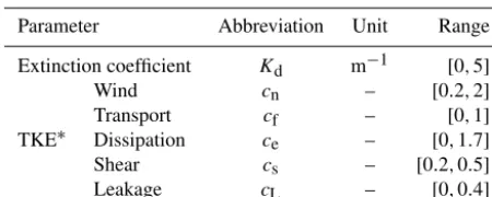
Table 1.Parameters of the Canadian Small Lake Model and their sampling ranges.

Parameter Abbreviation Unit Range

Extinction coefficient Kd m−1 [0,5]

TKE∗

Wind cn – [0.2,2]

Transport cf – [0,1]

Dissipation ce – [0,1.7]

Shear cs – [0.2,0.5]

Leakage cL – [0,0.4]

∗_{Turbulent kinetic energy budget.}

CSLM, shortwave extinction is exponential with depth fol-lowing Beer’s law, withKdidentified as thee-folding depth.

The turbulence subroutine in CSLM is used to determine the mixed layer depth; the depth over which active mixing occurs, homogenizing the temperature profile. This is the fi-nal step within the model before the temperature profile and fluxes are output. The change in mixed layer depth is calcu-lated by assessing the change in TKE. This change is deter-mined through the competition between energy input terms which act to increase the mixed layer depth and loss terms which act to decrease the depth of the mixed layer. Energy input terms include wind-driven stirring and buoyancy fluxes

Fq

, transport of TKE to the thermocline (Fi)which acts

to erode it, and shear production at the base of the mixed layer (Fs). Loss terms include energy dissipation (Fd),

en-trainment of deeper water at the thermocline Fpand sinks

of TKE within the mixed layer(FL). In this scheme the

mod-eled integrated TKE budget is used to determine the turbu-lence within a mixed layer of uniform properties and depth h(Imberger, 1985; Spigel et al., 1986). This is expressed as follows:

d dt

₁

2hEs

=h

2 dEs

dt + Es

2 dh

dt, (1)

where Es

2 is the average TKE per unit mass. To solve the

energy budget, the terms on the right-hand side are rewritten as the sum of relevant turbulent processes:

h 2

dEs

dt =Fq−Fd−Fi, (2)

Es

2 dh

dt =Fi+Fs−Fp−FL. (3)

This parameterization involves five empirical turbulent co-efficients (Table 1). With the exception of the entrainment term,Fp, the definition of each of the terms contains a

con-stant empirical coefficient: cnfor surface mechanical input,

ce for TKE dissipation,cffor TKE transport to the

thermo-cline,cs for shear production and cL for the sinks of TKE.

Experiments detailed in Spigel et al. (1986) yield a range of values forcn,cf,ceandcs. A set of consistent values was

cho-sen by Rayner (1980) and have been used subsequently by

Spigel et al. (1986) and MacKay (2012):cn=1.33,cs=0.2,

ce=1.15 andcf=0.25. MacKay (2012) chosecL=0.235

based on experimental data.

Both turbulent mixing andKddirectly control the output

of temperature and heat fluxes. In addition, there is also a considerable amount of uncertainty in both. In the case of the turbulent subroutine, the values of the empirical constants, while consistent, have never been investigated. The value of Kd, however, carries uncertainty due to limitations in its

mea-surement both spatially and temporally. Although measure-ment technology has long been available (Poole and Atkins, 1929), continuous measurements ofKdare, to the best of our

knowledge, relatively scarce despite the relative affordability of cosine collectors, perhaps currently the most widespread technology; see Frankovich et al. (2017) for a recent appli-cation. Also, point measurements can be taken through more or less direct proxies, such as the Secchi disk depth (Tyler, 1968) and dissolved organic compound (DOC) concentra-tions (Ask et al., 2009). The technology is in fact evolving (Chudyk and Flynn, 2015). Alas, despite the availability of measurement tools,Kdmight sometimes be an afterthought,

as in the case here presented, where it was determined from DOC concentrations.

2.1 The lake

Data from Landing Lake in Baker Creek (NWT, Canada; Fig. 1) were used to evaluate temperature profiles and heat fluxes produced by CSLM. Landing Lake is a small freshwa-ter lake with a surface area of 1.12 km2. While no compre-hensive bathymetry measurements have been taken on Land-ing Lake, depths in the main body of the lake durLand-ing installa-tions of thermistors and pressure transducers over the course of this study and others are consistently 4 m. The lake’s two southern arms are shallower, near 1.5 m, as can be seen by the change in colouration in Fig. 1. Concentrations of DOC are high, resulting in an expectedKdvalue of∼2 m−1(Spence

et al., 2003). Due to the shallow depth and high value ofKd,

the lake does not form a seasonal thermocline, but diurnal thermoclines were observed in the temperature data.

Meteorological, radiation and turbulent flux measurements were taken from a climate station installed on a bedrock out-crop island that was first described in Granger and Hedstrom (2011). This location provided fetch distances that ranged from 150 to 900 m. Data from the station were obtained for the open-water periods 2007–2009. Turbulent fluxes of sensible and latent heat (W m−2_{, positive upward from the}

were collected and processed at 30 min intervals using a dat-alogger (Campbell Scientific CR3000). Corrections to the eddy-covariance measurements include 2-D coordinate rota-tion (Baldocchi et al., 1988), air density fluctuarota-tions (Webb et al., 1980), sonic path length, high-frequency attenuation and sensor separation (Massman, 2000; Horst, 1997). Asso-ciated 30 min average meteorological observations included horizontal wind speed (m s−1) measured with a Met One 14A cup anemometer, air temperature (◦C) and relative humid-ity (%) measured with a Vaisala HMP45C thermohygrom-eter. Incoming and outgoing shortwave radiation (W m−2) were measured with paired upward- and downward-facing Li-Cor LI200S pyranometers. A Kipp and Zonen NRLite was mounted 1.04 m above the water to measure net radia-tion (W m−2). Because of the homogenous nature of the lake bathymetry, one vertical array of Onset pendant thermistors was deployed 300 m northeast of the island, measuring half-hourly water temperature at 4 depths (0, 0.5, 1, 2 m) in 2007 and 2008 and at 3 depths (0, 0.5, 1.5 m) in 2009.

3 Sensitivity analysis – an overview

When considering model-performance analysis, particularly in the case of complex models, it is important to note that one or more model parameters might exert more or less influence on one or more model outputs. Some of these parameters may be observable and/or measured while others may have dubious physical interpretation. How to specify model parameters is not a trivial issue (Gupta and Sorooshian, 1985; Stefanski, 1985; Wagener et al., 2003). Over-parameterization, parameter interactions, erro-neous evaluation data and computational errors are all causes of equifinality (Beven, 2006): different parameter-value com-binations yielding nigh-indistinguishable results. Sensitivity analysis (SA) provides a way to mitigate the equifinality is-sue by identifying the parameters that dominate model per-formance. Unimportant parameters may be used to reduce dimensionality, palliating equifinality with minimal impact on performance (Huang and Liang, 2006; van Werkhoven et al., 2008, 2009). Better constraints on important param-eters (e.g., through improved measurements) may result in uncertainty reduction.

There are many different approaches for SA; see Gan et al. (2014) and Song et al. (2015) for a thorough discus-sion. Song et al. (2015) in particular provide an exhaustive overview of the state-of-the-art. In general terms, SA meth-ods can be classified as global and local. Local measures as-sess model response by varying one parameter at a time while global measures vary several parameters simultaneously. Lo-cal measures do not account for possible parameter interac-tions but are computationally lighter since, all other condi-tions being equal, they require fewer evaluacondi-tions. The less demanding method is in fact differential SA, which uses

par-tial derivatives or finite differences at a location – parameter-value combination – of interest.

If the location of interest within the parameter space is not known a priori, a common occurrence given the equifi-nality issue, then random-sampling global SA measures are preferred. However, this necessitates more model evaluations since instead of varying just one parameter or looking at a specific location they are based on exploring the entirety of the feasible parameter space. The generalized likelihood uncertainty estimation (GLUE; Beven and Binley, 2014) is a global SA method that evolved from the work of Horn-berger and Spear (1981) and consists of randomly sampling the prior parameter space and evaluating the performance of the model at each random parameter-value vector, selecting behavioral (well-performing) vectors either after subjective thresholding (Li et al., 2010) or using measurement error as a splitting criteria: the limits-of-acceptability approach (Coxon et al., 2014).

The projection of the multidimensional parameter-value vectors into a plane defined by one of said parameters and the corresponding performance (“dotty plots”) can then be used to define a one-dimensional frequency distribution that is indicative of the parametric sensitivity. Furthermore, an estimate of the uncertainty of model simulations can be ob-tained by weighing them according to the performance, de-riving uncertainty bounds. The GLUE approach, however, is computationally inefficient, especially since strong informa-tion about prior parameter distribuinforma-tions is often unavailable and random uniform sampling required.

Computational performance of global SA can be im-proved using the design-of-experiment approach (Tong and Graziani, 2008), which consists of two steps. First, while still random, sampling is designed to efficiently cover the prior parameter space, or is tailored specifically for a given global SA method. Second, variation in model performance is at-tributed to the variation of different parameters; see Gan et al. (2014). The relative ranking of parameters and quantitative attribution of model–output variance might change depend-ing on the sampldepend-ing technique and global SA method (Gan et al., 2014).

Tong (2013) developed the PSUADE (Problem Solving environment for Uncertainty Analysis and Design Explo-ration) package that provides a collection of tools to perform uncertainty quantification and sensitivity analysis. PSUADE has been used to produce technical reports related to the mod-eling of explosives (Hsieh, 2006; Wemhoff and Hsieh, 2007), to the modeling of a two-dimensional interaction between soil and foundation structure (Tong and Graziani, 2008), and to the modeling of an electrostatic microelectromechanical system switch (Snow and Bajaj, 2010). Tong and Graziani (2008) use PSUADE to produce a book chapter exploring uncertainty quantification for multiphysics applications.

Table 3 in Song et al. (2015) for an overview of recent appli-cations), sometimes disregarding global SA in favor of local SA: e.g., most applications of PEST (Skahill and Doherty, 2006) where the number of calibration parameters can be re-duced using local SA.

The present study was based on a combination of three factors underlining its relevance: firstly, by building upon ex-isting literature that stresses the importance of lake clarity in modeling heat transfers (Heiskanen et al., 2015; Rose et al., 2016; Woolway et al., 2016) and evaluating against measured fluxes, as done by Deacu et al. (2012) for large lakes.

Secondly, while the difficulty in finding adequate param-eterizations for land-surface schemes has been recognized (Hogue et al., 2005; Duan et al., 2006; Demarty et al., 2005), and the importance of incorporating observational data has been underlined (Liu et al., 2005), little effective attention has been placed on uncertainty analysis in this kind of phys-ical modeling. Regarding lakes, inroads have been made, but with respect to water quality (Missaghi et al., 2013).

Thirdly, PSUADE is a recently available tool that provides the mechanisms to perform the kind of exhaustive SA pio-neered by Gan et al. (2014) that allows easy testing of dif-ferent methods within a single package and hence provides more robust results. Furthermore, quantifying the uncertainty in the connecting fluxes of the different components of a modular system (in this case a land-surface scheme) should be one of the first steps, often not performed, in an overall uncertainty assessment. This paper also represents a start in that direction. Our concrete objectives were to find the fol-lowing.

a. What were the parameters that dominated model perfor-mance, in terms of latent and sensible heat fluxes, eval-uated with two different objective functions, the Nash– Sutcliffe Efficiency (NSE; Nash and Sutcliffe, 1970) and the mean absolute error (MAE)?

b. What was the uncertainty in the modeled fluxes, which was quantified using the GLUE methodology?

3.1 SA methods

The purpose of this section is to describe without going into mathematical detail the different methods used for sensitivity analysis, emphasizing the assumptions each one makes. A formal description of the different methods can be found in Gan et al. (2014).

It should be kept in mind that there are different ways of categorizing SA methods (Song et al., 2015) and that there is no consensus regarding terminology (Razavi and Gupta, 2015). The methods used in this paper were all global – the combined effect of multiple parameters was considered – and the term “sensitivity” itself was meant as a ranking of the im-pact that model parameters had on model performance, ob-tained from comparison of observed and modeled data. In broad terms, the global SA methods applied are classified

as qualitative methods that provide a relative ranking of pa-rameter sensitivity and quantitative methods that attempt to explain how much of the variance in the model performance is explained by the variance in each individual parameter or combination of parameters.

3.1.1 Description

Besides their ability to screen the most important parame-ters, the common thread between qualitative methods is that they require relatively fewer model runs, compared to quan-titative ones. They might however differ in their concep-tual approach. For instance the Spearman rank correlation (SPEAR; Spearman, 1904) and the standard regression coef-ficient (SRC; Galton, 1886) share a conceptual framework: they are regression methods, that simulate performance as a linear combination of parameter values.

SPEAR bases its sensitivity rankings on the degree of lin-ear correlation between each individual parameter and per-formance. SRC stipulates a predictive model as a linear com-bination of all parameter values. The SRC value for each parameter is obtained by normalizing the coefficients of the predictive model. It should be noted that the predictive model need not be linear, but often is, as was the case here. A down-side of the regression methods is that their robustness is de-pendent on their predictive capability (Yang, 2011).

Another conceptual approach is to view the partial deriva-tives of model performance with respect to model parame-ters as indicators of parameter sensitivity: the steeper the re-sponse surface around a given point, the more sensitive the parameter in that region. An analytical solution would allow explicit evaluation over the entire parameter space but that is a practical impossibility for most, if not all, models. Instead numerical approximations are computed at selected points and averaged to give an indication of the relative sensitiv-ity of the model parameters. This is the Morris one-at-a-time (MOAT; Morris, 1991) approach. The sensitivity is evaluated by computing both the mean (MOAT-1) and the standard de-viation (MOAT-2) of the partial derivatives at selected sam-ple points. It is a robust method in the sense that no assump-tions are made for the relaassump-tionship between model parameter values and performance.

the response surface, and will produce reliable results only if those assumptions are met.

MARS is an extension of the concept of linear models to a multidimensional setting and consists of fitting, through lin-ear regression, (hyper-)planes to the response surface of the model. It is in essence an extension of the recursive parti-tioning approach to regression: determining the breaks for the piecewise linear fits from the data. The relative impor-tance of the parameters is determined by dropping them in turn from the regression and reevaluating the performance: the bigger the drop in performance, the more important the parameter.

DT was originally developed for time series modeling, the basic premise being that a chaotic dynamic system can be reconstructed from sequences of observations of its state (Pi and Peterson, 1994). Eirola et al. (2008) is an example of the DT method parameter-screening tool: the subset of parameters that minimize the variance in the noise (differ-ence between observed and modeled performance) are seen as the most sensitive ones. Testing all possible parameter subsets is computationally infeasible and the PSUADE pack-age chooses the best 50 subsets for scoring. Furthermore, the method itself is computationally demanding since it might require operations on large matrices and can be affected by numerical instabilities.

The premise of SOT is that model parameters can be used to simulate performance based on a binary decision tree: each parameter can be used to partition the parameter space into two areas with different responses and the sum of all different partitions used to predict performance. The number and par-tition setup is determined through a recursive binary division of the parameter space. The required number and ordering of the partitions is evaluated by comparing the residuals be-tween the tree-predicted performance and the computed one, until a convergence criteria is met. The relative importance of each parameter is proportional to the number of nodes in the tree that include that parameter.

GP assumes performance follows a multivariate normal distribution, characterized by the means and the covariance matrix of the different parameters. While the means of the parameters are dependent on their relative scalings, the nor-malized covariances are not and this allows comparison of the degree of change in the response along the different di-mensions. The relative degrees of change along the different dimensions are an indicator of parameter sensitivity.

These qualitative measures do not explain how much of the performance variance is due to a given parameter (or parame-ter inparame-teraction). Quantitative measures such as Fourier ampli-tude test (FAST; Cukier et al., 1973), McKay main (McKay-1) and two-way (McKay-2) interaction analyses (McKay et al., 1999), and Sobol sensitivity indices (Sobol, 1990, 2001) provide such quantitative assessment. All quantitative methods are variance-based methods that use an ANOVA-like decomposition (Fisher, 1925) to identify the subset of

parameters that dominate performance simulation, but differ in the way performance is simulated.

In FAST, model performance is expressed as a Fourier series, incorporating different model parameters. Since the model is a function of several parameters, a multidimensional integral is required to evaluate the Fourier coefficients. This is solved by making it one-dimensional through application of the ergodic theorem. Of the methods listed here, it is the one that requires the least amount of model runs.

The McKay method attempts to find the subset of param-eters that better approximates the performance variance by computing the ratio between the performance variance for a subset of parameters and the performance variance for all parameters, which is a measure of the relative importance of each subset. The performance variance is computed through random sampling of the parameter space, making the method nonparametric The subset that maximizes the ratio is consid-ered the most sensitive subset. McKay et al. (1999) extended the concept to account for two-way parameter interactions (McKay-2) and their effect on the performance variance, as-suming the parameters to be uncorrelated.

In the Sobol method, model performance is decomposed into summands of functions of the parameters, in increas-ing order of dimensionality. Assumincreas-ing orthogonality of all summands permits expression of the performance in terms of a sum of conditional expected values. Further assuming that said sum is a square integrable makes it possible to equate performance variance to a sum of variances and co-variances of model parameters. The effect of model parame-ters on model output can then be decomposed into first-order indexes, where the contribution of the variance of each indi-vidual parameter on model output can be quantified and can also include the interactions of model parameters (the co-variances). The number of interactions to include range from second order, where just two-way parameter interactions are included, to total effect, where all possible interactions are accounted for. The final result is a ratio that shows how much of the output variance can be explained by a parameter or combination of parameters.

3.2 Uncertainty analysis with GLUE

GLUE (Beven and Binley, 2014) is a widely applied method, particularly in hydrology, used to evaluate parametric sensi-tivity and to quantify parametric uncertainty. This paper fo-cuses on the latter aspect in order to provide an estimate of the impact of uncertainty on the modeled fluxes.

Table 2.Sensitivity analysis methods. Qualitative methods in black font. Quantitative methods in bold font.

SA method Abbreviation Source

Correlation analysis SPEAR Spearman (1904)

Regression analysis SRC Galton (1886)

Morris one-at-a-time screening MOAT Morris (1991)

Sum-of-trees screening SOT Breiman et al.(1984)

Gaussian process screening GP Gibbs and Mackay (1997)

Multivariate adaptive regression splines screening MARS Friedman (1991)

Delta-test screening DT Pi and Peterson (1994)

Fourier amplitude sensitivity test FAST Cukier et al. (1973) Sobol sensitivity indices SOBOL Sobol (1990, 2001)

bounds extracted from weighted simulations, e.g., at each time step the 0.05 and 0.95 percentiles of the likelihood-weighted simulations can be extracted and considered to be the 95 % confidence interval.

To each combination of parameter values there is a cor-responding performance. The projection of the (multidimen-sional) parameter values against performance along one di-mension, or parameter axis, produces what are commonly known as “dotty plots” which can give an idea of paramet-ric sensitivity (Beven, 2006).

4 Methods and performance metrics

The CSLM simulates heat-transfer fluxes – latent and sensi-ble heat – at the boundary between lake surface and the at-mosphere. The model was run with half-hourly forcings and the resulting simulations were temporally aggregated to eval-uate against daily flux data, which were obtained through in-tegration of hourly eddy-covariance measurements. The ag-gregation was necessary because of inherent limitations of the higher-frequency daily covariance data that were avail-able for the period 12 June–18 October 2007. Two perfor-mance metrics were used for the evaluation, MAE and NSE:

MAE=

Pn

i=1|Oi−Si|

n , (4)

NSE=1−

Pn

i=1(Oi−Si)2

Pn

i=1 Oi−O

2, (5)

wherenis the number of time steps at which the model was evaluated,Oi was the observed value at time stepi,Si was the simulated value at time stepi, andOis the mean of the observed values. The rationale behind the choice was to con-trast the propensity of NSE to prioritize better-fitting high values (Krause et al., 2005), sometimes to the detriment of other ranges, by using MAE as a contrasting metric, less dependent on high-value fit. The entire period with avail-able data was used for the computation of the performance measures. The metrics were computed after aggregating the hourly data to a daily time step.

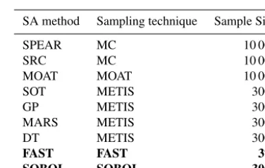
Table 3.Setup for SA. Qualitative methods in black font. Quantita-tive methods in bold font.

SA method Sampling technique Sample Size

SPEAR MC 10 000

SRC MC 10 000

MOAT MOAT 10 000

SOT METIS 3000

GP METIS 3000

MARS METIS 3000

DT METIS 3000

FAST FAST 373

SOBOL SOBOL 3000

Sampling techniques: (a) MC: uniform sampling, (b) MOAT: designed specifically for MOAT, (c) METIS: space-filling method, (d) FAST: designed specifically for FAST and (e) SOBOL: designed specifically for SOBOL. See Gan et al. (2014) for a description of the sampling methods.

MAE and NSE were the basis of all tested SA methods (Table 2). The PSUADE (Tong, 2013) package is a tool that assembles SA methods under a unified computational frame-work, thus facilitating exhaustive testing in the vein of Gan et al. (2014), who tested the impact of sampling, in terms of frequency and technique, and different SA methods in the identification of sensitive parameters for a hydrological model. The general procedure for PSUADE is as follows: (a) generate random samples, (b) run the model and compute the performance for all the samples and (c) compute SA met-rics from the obtained performances. The performance used was the average performance for the simulation of latent and sensible heat.

Kd

c n

cf

ce

cs

cL

MOAT-1 MOAT-2

Figure 2.Comparison of the relative sensitivity of a subset of the parameters of the Canadian Small Lake Model, using the Nash– Sutcliffe performance to evaluate the model.

space and some are better suited than others depending on the purpose (McKay et al., 1979).

The CSLM was sufficiently fast to run, less than a sec-ond for 128 days of half-hourly data, so that the number of simulations required by the different methods was not a lim-itation. Therefore we ran as many simulations as necessary to obtain consistent results (Table 3). The choice of sampling method was based on those used by Gan et al. (2014) in their experiment.

Seven qualitative and two quantitative SA methods were tested to identify the sensitive parameters in CSLM. The pa-rameters chosen for the test are the ones deemed a priori to have physical significance for the thermodynamic function-ing of the lake. The range of the parameters was based on physically plausible values (Table 1).

Finally, in order to broadly estimate the impact of paramet-ric uncertainty on heat-flux simulation, the GLUE procedure was applied to CSLM for the parameters, and ranges, listed in Table 1. A total of 1 million simulations were performed and the top 10 % selected as behavioral in order to compute the uncertainty bounds. For MAE, the lower the value, the better the performance, and therefore the inverse of the computed MAE was used as the likelihood when performing GLUE. The NSE values were used unmodified for the weighting.

5 Results

5.1 Qualitative measures

We first performed SA using qualitative methods (Table 2) and obtained a ranking of the model parameters in terms of sensitivity. The results were presented as a color map where the darker tones indicate larger sensitivity (Figs. 2

Figure 3.Comparison of the relative sensitivity of a subset of the parameters of the Canadian Small Lake Model, using the Mean Av-erage Error to evaluate the model.

and 3). Near unanimity was reached, for both MAE and NSE, in identifyingKd, the light attenuation coefficient, as

the most sensitive parameter for the simulation of heat fluxes (Table 4). The sole exceptions were the SPEAR and SRC methods. A strong assumption for both these methods is that model response varies linearly with input, which is almost never the case for environmental models (Beven, 2006): re-sponse surfaces tend to be very complicated (Duan et al., 2006). Another method with strong prior assumptions about model response is GP, which fits the response surface to a multivariate normal distribution. Global model response is seldom normal due to the overall complexity of the response surface, but if the response is locally linear in a region of the parameter space, then the approximation might be adequate (Kuczera, 1990).

A physical explanation of the results obtained here, that pinpointKdas the most sensitive parameter in terms of

sim-ulating heat transfers, can be inferred from the fact that the lake is shallow and therefore it is perhaps not surprising that the turbulent transfer coefficients exert no major impact on such processes. A similar analysis – not shown here – study-ing parameter sensitivity with respect to the thermal structure of the lake also highlighted the importance of theKd

param-eter for the thermal balance of the lake. 5.2 Quantitative measures

It was evident (Figs. 2 and 3) that model response, in terms of simulating heat fluxes, is dependent on the value of the Kdparameter. None of the qualitative measures, however, do

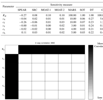
Table 4.Parameter sensitivity rankings of different qualitative sensitivity analysis methods.

Parameter Sensitivity measure

SPEAR SRC MOAT-1 MOAT-2 MARS SOT DT GP

Kd −0.27 0.08 0.10 0.10 100.00 1.00 1.00 100.00

cn −0.04 0.02 0.01 0.01 10.00 0.06 0.27 5.66

cf −0.26 −0.06 0.01 0.03 10.00 0.07 0.23 1.37

ce −0.00 −0.01 0.00 0.02 3.00 0.01 0.24 0.14

cs −0.02 −0.02 0.00 0.01 4.00 0.02 0.21 0.05

cL 0.11 0.03 0.01 0.02 5.00 0.03 0.22 0.46

Kd

cn

cf

ce

cs

cL

Kd cn

cs

ce

cf cL

Figure 4.Two-way correlation between selected parameters of the Canadian Small Lake Model. This indicates how much the value of a given parameter is dependent on the value of another one to produce good simulations. The mean absolute error was used to evaluate the model. McKay-2 (McKay et al., 1999) was used to evaluate the correlation.

McKay-2 (Figs. 4 and 5) ranked two-way correlations, which is the sum of first- and second-order effects of dif-ferent parameter combinations on performance. The impor-tance ofKdwas once again incontestable: no other parameter

combinations besides those containingKdwere more

impor-tant for the simulation of heat transfer. Put in another way, this also meant that Kd by itself was more important than

any other parameter combination. This is especially reveal-ing since even parameters with low main-effect may have significant effect on performance through their interaction with other parameters, but here all evidence points toKdas

the main culprit.

In fact, from first-order to total-order effects (Figs. 6 and 7), it was Kd that dominated model response both in

qualitative and quantitative terms. There was, however, some difference in the first-order effects estimated with either FAST and SOBOL-1 (Figs. 6 and 7). A conceptual differ-ence between the two is that FAST approximates model out-put as a Fourier series, which implies that a better fit might be obtained in time series with a degree of seasonality, whereas

SOBOL only relies on expected values computed from a ran-dom sample of the data. The downside of the SOBOL anal-ysis is that it requires many more simulations to reach con-sistent results. There was no reason to expect seasonality for this dataset, as it comprised less than 1 year of continuous data. The model was lightweight enough that computation time was not a factor for the SOBOL analysis. Therefore the SOBOL results, which show a larger importance forKd,

were probably more indicative of the efficacy of parameter sensitivity.

5.3 GLUE

Kd

cn

cf

ce

cs

cL

Kd cn

cs

ce

cf cL

Figure 5.Two-way correlation between selected parameters of the Canadian Small Lake Model. This indicates how much the value of a given parameter is dependent on the value of another one to produce good simulations. The Nash–Sutcliffe performance was used to evaluate the model. McKay-2 (McKay et al., 1999) was used to evaluate the correlation.

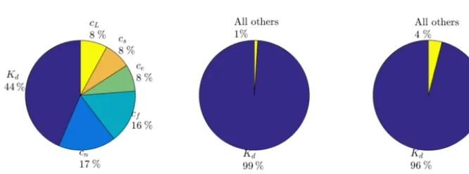
Figure 6.First- and total-order effects indicating the sensitivity of the model parameters on model performance. First-order effects ac-count for parameters independently whereas second-order effects take include possible correlations between parameters. First-order effects were computed with the FAST and Sobol-1 methods. Second-order effects were computed using the Sobol-tmethod. The Nash–Sutcliffe performance was used to evaluate the model.

number of simulations performed, the results were a robust indicator of the possible output range: the ability of the model to reproduce observed data.

The importance of Kd is once again highlighted in the

dotty plots (Fig. 9): it was the only parameter that perfor-mance was sensitive to. The value of the turbulent transport parameters had little impact on model performance.

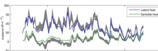
Finally, there is a trade-off in the simulation of latent and sensible heat (Figs. 8 and 10), and even considering the generous behavioral threshold that was set, the uncertainty bounds did not always encompass measurements (Fig. 8).

6 Conclusions

Most SA methods pinpointed Kd as the most sensitive

pa-rameter in terms of simulating latent and sensible heat fluxes.

The exceptions were those which had the strongest assump-tions with respect to the nature of model response: SPEAR and SRC assume linearity between input (model parameter) and response (performance measure), which was not the case for CSLM. Somewhat surprisingly, GP, which also makes as-sumptions about the shape of the response surface and con-siders it Gaussian, also showedKdto be the most sensitive

parameter. This was either a false positive or the response surface might have been locally linear, thus justifying the normality assumption (Williams, 1998). None of the other methods makes such strong assumptions about the nature of the response surface, although localized fitting does occur: e.g., stepwise linear for MARS.

This predominance ofKdis perhaps not surprising given

Wool-Figure 7.First- and total-order effects indicating the sensitivity of the model parameters on model performance. First-order effects account for parameters independently whereas second-order effects take include possible correlations between parameters. First-order effects were computed with the FAST and Sobol-1 methods. Second-order effects were computed using the Sobol-tmethod. The mean absolute error was used to evaluate the model.

Ir

ra

di

an

ce

(

W

m

2)

heat

Figure 8.The 5 and 95 % uncertainty bounds for the heat fluxes, obtained from the GLUE global sensitivity method. The Nash–Sutcliffe performance was used to evaluate the model for the 2007 open-water season.

way et al., 2016; Rose et al., 2016). Given the complex and intertwined processes that can affect light penetration, such as browning waters (Roulet and Moore, 2006) and ecosystem function (Tilzer, 1983, 1988; Mazumder et al., 1990; Rinke et al., 2010), a single measurement of its value might prove insufficient. It might be necessary to rely on continuous mea-surement in order to improve modeling, either through adher-ence to a parsimony principle (its value need not be modeled if actually measured) or stemming from the need to evaluate the complex processes influencing its value.

The light extinction coefficient is the only parameter con-sidered in this analysis that is directly measurable (Table 1). Being able to measure the most sensitive parameter is a def-inite advantage: it allows the number of parameters needing calibration to be confidently reduced. Furthermore, sinceKd

is so predominant in terms of model performance that mak-ing it a measured instead of a calibrated quantity should fa-cilitate further model evaluation, whatever variability in the performance that was not a function of Kd should become

easier to quantify and analyze since it would not be obfus-cated byKd’s predominance.

With respect to large-scale applications, such as climate modeling and land-surface schemes, measuring Kd for

ev-ery lake might be a practical impossibility, but its importance

should be stressed and further research devoted to assess its temporal and spatial variability. Remote sensing might pro-vide a solution to lack of in situ measurements and is in fact used to provide estimates of the Secchi depth (Torbick et al., 2013), a proxy for the light extinction coefficient.

The model did not perform equally well at different time periods (Fig. 8) andKd is known to vary over time (Rinke

et al., 2010). A first step into assessing causality between these two factors would be to continually measure Kd, at

least at a daily time step. Such measurements have proved useful in evaluating turbulent transfers over large lakes (Deacu et al., 2012).

There is often a disconnect between experimentalists and computer modelers (Seibert and McDonnell, 2002, 2013). The conceptual framework behind the present study is a tes-tament to an improvement of those dialogues: the undertaken modeling approach was based on data from an observation station that was explicitly established to support testing of hydrometeorological models over lakes. Such new data fa-cilitated the analysis performed here and it must be stressed that measuringKdwas not part of the objectives of the field

Kd cn

cf ce

cL

cs

Kd cn

cf ce

cL

cs

W/m

2

2

(W

m

2)

(W

m

2)

Sensible heat Latent heat

Figure 9.Mean absolute error for sensible and latent heat fluxes, from the GLUE simulations. Each dot represents a simulation with ran-dom parameters. Theyaxis shows heat flux (W m−2) and thexaxis is the parameter value. Results were similar for the Nash–Sutcliffe performance.

M

A

E

la

te

n

t h

ea

t

(W

m

-2)

MAE sensible heat (W m-2₎

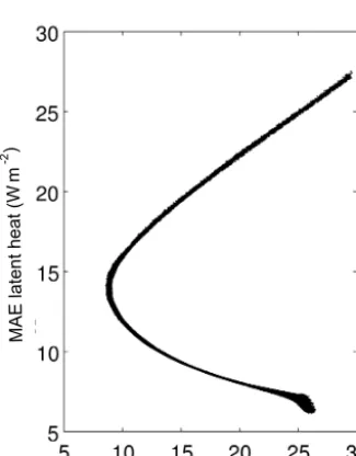
Figure 10.Latent vs. sensible heat (W m−2) for behavioral (well-performing) simulations. Each dot was the output from a random simulation. The mean absolute error was used to evaluate the model. Results were similar for the Nash–Sutcliffe performance.

The limitations of SA methods are tightly related to the curse of dimensionality (Saltelli and Annoni, 2010). All SA methods obviate the issue by randomly sampling the param-eter space, implicitly assuming results to be representative of the entire space. This is especially problematic in high-dimensional spaces, where even the simplest of models might face prohibitive computational costs and even the most so-phisticated sampling schemes are limited in their coverage of the parameter space.

The uncertainty bounds obtained from the GLUE analy-sis are nothing but subjective since the behavioral threshold

was arbitrarily set for the top 10 % simulations. Even with this rather lenient criteria, the bounds did not encompass all observations, especially for sensible heat (Fig. 8). This might be due to the tradeoffs between latent and sensible heat sim-ulation (Fig. 10) and the chosen performance measures, but might also stem from inadequate process representation. The clear tradeoffs in performance for latent and sensible heat might be influenced by the fact that while the CSLM surface energy balance is a strongly nonlinear function of the surface skin temperature, both the sensible and latent heat fluxes are linear terms in this relationship. All other things being equal, this leads to a direct tradeoff between them: the capacity of the model to simulate one of the terms is inversely propor-tional to its ability to simulate the other; see Fig. 10.

PSUADE is a powerful package that facilitates SA by pro-viding a wealth of approaches and presents an opportunity that evaluate their appropriateness, a factor of special im-portance since they are based on different conceptual pre-cepts. Overall the results might depend on the quality of the sampling, but that was not a factor here since the model was lightweight enough for the number of runs not to be a lim-iting factor. This will definitely not be the case with more complex models. If runtime is an issue methods like GLUE become nonviable. FAST, however, requires relatively fewer simulations to reach consistent results, but makes assump-tions about the nature of the response surface. The latter is true for most RSM methods: the robustness of the results de-pends on the validity of these assumptions.

being numerical instabilities, especially when a large num-ber of parameters is involved. All methods might fail in the presence of singularities or discontinuities in the response surface and if they give the right answer it might be for the wrong reasons.

In all, to recommend a preferred method is difficult and very much depends on the nature of the problem. If the pop-ularity of their use is an indicator, then the MOAT and RSM approaches are the most used in the literature (Song et al., 2015). It is the authors’ opinion that the SOBOL method provides the most complete insight but is difficult to apply in high-dimensional spaces and is prone to numerical insta-bilities.

Despite the shortcomings, the answer to our original ques-tion was clear:Kdis undeniably the most sensitive parameter

in the simulation of heat fluxes.

Data availability. The observations are archived at Environment and Climate Change Canada and are available from the authors upon request.

Competing interests. The authors declare that they have no conflict of interest.

Acknowledgements. Financial support from the Canada Excellence Research Chair in Water Security and the Natural Science and Engineering Research Council’s Changing Cold Regions Network is gratefully acknowledged. We also acknowledge support from Nordforsk Nordic eScience Globalisation Initiative (NeGI) project 74306 “An open-access generic e-platform for environmental model-building at the river-basin scale“.

Edited by: Dimitri Solomatine Reviewed by: two anonymous referees

References

Ask, J., Karlsson, J., Persson, L., Ask, P., Byström, P., and Jansson, M.: Terrestrial organic matter and light penetration: Effects on bacterial and primary production in lakes, Limnol. Oceanogr., 54, 2034–2040, https://doi.org/10.4319/lo.2009.54.6.2034, 2009. Baldocchi, D. D., Hicks, B. B., and Meyers, T. P.: Measuring

biosphere-atmosphere exchanges of biologically related gases with micrometeorological methods, Ecology, 69, 1331–1340, https://doi.org/10.2307/1941631, 1988.

Bates, G. T., Giorgi, F., and Hostetler, S. W.: Toward the Simula-tion of the Effects of the Great Lakes on Regional Climate, Mon. Weather Rev., 121, 1373–1387, https://doi.org/10.1175/1520-0493(1993)121<1373:TTSOTE>2.0.CO;2, 1993.

Beven, K.: A manifesto for the equifinality thesis, J. Hydrol., 320, 18–36, https://doi.org/10.1016/j.jhydrol.2005.07.007, 2006. Beven, K. and Binley, A.: GLUE: 20-years on, Hydrol. Proc., 28,

5897–5918, https://doi.org/10.1002/hyp.10082, 2014.

Beven, K. and Germann, P.: Macropores and water flow in soils revisited, Water Resour. Res., 49, 3071–3092, https://doi.org/10.1002/wrcr.20156, 2013.

Beven, K. and Lamb, R.: The uncertainty cascade in model fusion, Geological Society, London, Special Publications, 408, 255–266, https://doi.org/10.1144/SP408.3, 2014.

Beven, K. and Westerberg, I.: On red herrings and real herrings: Disinformation and information in hydrological inference, Hy-drol. Proc., 25, 1676–1680, https://doi.org/10.1002/hyp.7963, 2011.

Blanken, P. D., Rouse, W. R., Culf, A. D., Spence, C., Boudreau, L. D., Jasper, J. N., Kochtubajda, B., Schertzer, W. M., Marsh, P., and Verseghy, D.: Eddy covariance mea-surements of evaporation from Great Slave Lake, North-west Territories, Canada, Water Resour. Res., 36, 1069–1077, https://doi.org/10.1029/1999WR900338, 2000.

Blanken, P. D., Spence, C., Hedstrom, N., and Lenters, J. D.: Evaporation from Lake Superior: 1. Physical con-trols and processes, J. Great Lakes Res., 37, 707–716, https://doi.org/10.1016/j.jglr.2011.08.009, 2011.

Breiman, L., Friedman, J., Stone, C., and Olshen, R.: Classifica-tion and Regression Trees, The Wadsworth and Brooks-Cole statistics-probability series, Taylor & Francis, 368 pp., 1984. Cael, B. B. and Seekell, D. A.: The size-distribution of Earth’s lakes,

Sci. Rep.-UK, 6, 29633, https://doi.org/10.1038/srep29633, 2016.

Chipman, H. A., George, E. I., and McCulloch, R. E.: BART: Bayesian additive regression trees, Ann. Appl. Stat., 6, 266–298, https://doi.org/10.1214/09-AOAS285, 2012.

Chudyk, W. and Flynn, K. F.: Fiber optic light sensor, Environ. Monit. Assess., 187, 1–7, https://doi.org/10.1007/s10661-015-4597-0, 2015.

Clark, M. P. and Kavetski, D.: Ancient numerical daemons of conceptual hydrological modeling: 1. Fidelity and efficiency of time stepping schemes, Water Resour. Res., 46, W10510, https://doi.org/10.1029/2009WR008894, 2010.

Coxon, G., Freer, J., Wagener, T., Odoni, N. A., and Clark, M.: Diagnostic evaluation of multiple hypotheses of hy-drological behaviour in a limits-of-acceptability framework for 24 UK catchments, Hydrol. Proc., 28, 6135–6150, https://doi.org/10.1002/hyp.10096, 2014.

Cukier, R. I., Fortuin, C. M., Shuler, K. E., Petschek, A. G., and Schaibly, J. H.: Study of the sensitivity of coupled reaction sys-tems to uncertainties in rate coefficients. I Theory, J. Chem. Phys., 59, 3873–3878, https://doi.org/10.1063/1.1680571, 1973. Deacu, D., Fortin, V., Klyszejko, E., Spence, C., and Blanken, P. D.: Predicting the Net Basin Supply to the Great Lakes with a Hy-drometeorological Model, J. Hydrometeorol., 13, 1739–1759, https://doi.org/10.1175/JHM-D-11-0151.1, 2012.

Demarty, J., Ottlé, C., Braud, I., Olioso, A., Frangi, J. P., Gupta, H. V., and Bastidas, L. A.: Constraining a physically based Soil-Vegetation-Atmosphere Transfer model with surface water content and thermal infrared brightness temperature measure-ments using a multiobjective approach, Water Resour. Res., 41, W01011, https://doi.org/10.1029/2004WR003695, 2005. Downing, J. A., Prairie, Y. T., Cole, J. J., Duarte, C. M., Tranvik,

distribu-tion of lakes, ponds, and impoundments, Limnol. Oceanogr., 51, 2388–2397, https://doi.org/10.4319/lo.2006.51.5.2388, 2006. Duan, Q., Schaake, J., Andréassian, V., Franks, S., Goteti,

G., Gupta, H., Gusev, Y., Habets, F., Hall, A., Hay, L., Hogue, T., Huang, M., Leavesley, G., Liang, X., Nasonova, O., Noilhan, J., Oudin, L., Sorooshian, S., Wagener, T., and Wood, E.: Model Parameter Estimation Experiment (MOPEX): An overview of science strategy and major results from the second and third workshops, J. Hydrol., 320, 3–17, https://doi.org/10.1016/j.jhydrol.2005.07.031, 2006.

Eggermont, H. and Martens, K.: Preface: Cladocera crustaceans: Sentinels of environmental change, Hydrobiologia, 676, 1–7, https://doi.org/10.1007/s10750-011-0908-9, 2011.

Eirola, E., Liitiäinen, E., Lendasse, A., Corona, F., and Verleysen, M.: Using the Delta test for variable selection, Proceedings of ESANN 2008 European Symposium on Artificial Neural Net-works, 25–30, 2008.

Elçi, ¸S.: Effects of thermal stratification and mixing on reservoir water quality, Limnology, 9, 135–142, https://doi.org/10.1007/s10201-008-0240-x, 2008.

Fisher, R. A.: Statistical methods for research workers, Oliver & Boyd, Edinburgh: Tweedale Court, 1925.

Frankovich, T. A., Rudnick, D. T., and Fourqurean, J. W.: Light attenuation in estuarine mangrove lakes, Estuar. Coast. Shelf S., 184, 191–201, https://doi.org/10.1016/j.ecss.2016.11.015, 2017. Friedman, J. H.: Multivariate Adaptive Regression Splines, Ann.

Stat., 19, 1–67, 1991.

Galton, F.: Regression Towards Mediocrity in Heredi-tary Stature, J. R. Anthropol. Inst. G., 15, 246–263, https://doi.org/10.2307/2841583, 1886.

Gan, Y., Duan, Q., Gong, W., Tong, C., Sun, Y., Chu, W., Ye, A., Miao, C., and Di, Z.: A comprehensive evaluation of various sensitivity analysis methods: A case study with a hydrological model, Environ. Model. Softw., 51, 269–285, https://doi.org/10.1016/j.envsoft.2013.09.031, 2014.

Gibbs, M. and MacKay, D. J. C.: Efficient implementation of Gaus-sian processes, Tech. rep., Cavendish Lab., Cambridge, UK, 1997.

Granger, R. J. and Hedstrom, N.: Modelling hourly rates of evap-oration from small lakes, Hydrol. Earth Syst. Sci., 15, 267–277, https://doi.org/10.5194/hess-15-267-2011, 2011.

Gupta, V. and Sorooshian, S.: The relationship between data and the precision of parameter estimates of hydrologic models, J. Hy-drol., 81, 57–77, https://doi.org/10.1016/0022-1694(85)90167-2, 1985.

Halldin, S., Gryning, S.-E., Gottschalk, L., Jochum, A., Lundin, L.-C., and Van de Griend, A.: Energy, water and carbon ex-change in a boreal forest landscape – NOPEX experiences, Agr. Forest Meteorol., 98–99, 5–29, https://doi.org/10.1016/S0168-1923(99)00148-3, 1999.

Heiskanen, J. J., Mammarella, I., Ojala, A., Stepanenko, V., Erkkilä, K. M., Miettinen, H., Sandström, H., Eugster, W., Leppäranta, M., Järvinen, H., Vesala, T., and Nordbo, A.: Ef-fects of water clarity on lake stratification and lake-atmosphere heat exchange, J. Geophys. Res.-Atmos., 120, 7412–7428, https://doi.org/10.1002/2014JD022938, 2015.

Hogue, T. S., Bastidas, L., Gupta, H., Sorooshian, S., Mitchell, K., and Emmerich, W.: Evaluation and Transferability of the Noah

Land Surface Model in Semiarid Environments, J. Hydrometeo-rol., 6, 68–84, https://doi.org/10.1175/JHM-402.1, 2005. Hornberger, G. and Spear, R.: An approach to the preliminary

anal-ysis of environmental systems, J. Environ. Manage., 12, 7–12, https://doi.org/10.1016/S0272-4944(89)80026-X, 1981. Horst, T. W.: A simple formula for attenuation of eddy fluxes

mea-sured with first-order-response scalar sensors, Bound.-Lay. Me-teorol., 82, 219–233, https://doi.org/10.1023/A:1000229130034, 1997.

Hsieh, H.: Application of the PSUADE tool for sensitivity analysis of an Engineering simulation, Tech. rep., Lawrence Livermore National Laboratory, Livermore, CA, 2006.

Huang, M. and Liang, X.: On the assessment of the impact of reduc-ing parameters and identification of parameter uncertainties for a hydrologic model with applications to ungauged basins, J. Hy-drol., 320, 37–61, https://doi.org/10.1016/j.jhydrol.2005.07.010, 2006.

Imberger, J.: The diurnal mixed layer, Limnol. Oceanogr., 30, 737– 770, https://doi.org/10.4319/lo.1985.30.4.0737, 1985.

Kalff, J. Downing, J. A.: Limnology: Inland water ecosystems, Up-per Saddle River, NJ, Prentice Hall, 2nd Edn., 2002.

Koster, R. D. and Suarez, M. J.: Modeling the land surface boundary in climate models as a composite of independent vegetation stands, J. Geophys. Res.-Atmos., 97, 2697–2715, https://doi.org/10.1029/91JD01696, 1992.

Koster, R. D., Suarez, M. J., Ducharne, A., Stieglitz, M., and Kumar, P.: A catchment-based approach to modeling land surface processes in a general circulation model: 1. Model structure, J. Geophys. Res.-Atmos., 105, 24809–24822, https://doi.org/10.1029/2000JD900327, 2000.

Krause, P., Boyle, D. P., and Bäse, F.: Comparison of different effi-ciency criteria for hydrological model assessment, Adv. Geosci., 5, 89–97, https://doi.org/10.5194/adgeo-5-89-2005, 2005. Kuczera, G.: Assessing hydrologic model nonlinearity

us-ing response surface plots, J. Hydrol., 118, 143–161, https://doi.org/10.1016/0022-1694(90)90255-V, 1990.

Kundzewicz, Z. W. and Stakhiv, E. Z.: Are climate models “ready for prime time” in water resources management applications, or is more research needed?, Hydrol. Sci. J., 55, 1085–1089, https://doi.org/10.1080/02626667.2010.513211, 2010.

Li, L., Xia, J., Xu, C.-Y., and Singh, V.: Evaluation of the subjective factors of the GLUE method and compar-ison with the formal Bayesian method in uncertainty as-sessment of hydrological models, J. Hydrol., 390, 210–221, https://doi.org/10.1016/j.jhydrol.2010.06.044, 2010.

Liu, Y., Gupta, H. V., Sorooshian, S., Bastidas, L. A., and Shuttleworth, W. J.: Constraining Land Surface and At-mospheric Parameters of a Locally Coupled Model Us-ing Observational Data, J. Hydrometeorol., 6, 156–172, https://doi.org/10.1175/JHM407.1, 2005.

Ljungemyr, P., Gustafsson, N., and Omstedt, A.: Parameterization of lake thermodynamics in a high-resolution weather forecasting model, Tellus A, 48, 608–621, https://doi.org/10.1034/j.1600-0870.1996.t01-4-00002.x, 1996.

MacKay, M.: A process-oriented small lake scheme for coupled cli-mate modeling applications, J. Hydrometeorol., 13, 1911–1925, https://doi.org/10.1175/JHM-D-11-0116.1, 2012.

J. D., Litchman, E., MacIntyre, S., Marsh, P., Melack, J., Mooij, W. M., Peeters, F., Quesada, A., Schladow, S. G., Schmid, M., Spence, C., and Stokesr, S. L.: Modeling lakes and reser-voirs in the climate system, Limnol. Oceanogr., 54, 2315–2329, https://doi.org/10.4319/lo.2009.54.6_part_2.2315, 2009. Manabe, S.: Climate and the ocean circulation – II. The atmospheric

circulation and the effect of heat transfer by ocean currents, Mon. Weather Rev., 97, 775–805, https://doi.org/10.1175/1520-0493(1969)097<0775:CATOC>2.3.CO;2, 1969.

Massman, W. J.: A simple method for estimating frequency re-sponse corrections for eddy covariance systems, Agr. For-est Meteorol., 104, 185–198, https://doi.org/10.1016/S0168-1923(00)00164-7, 2000.

Mazumder, A., Taylor, W. D., McQueen, D. J., and Lean, D. R.: Effects of Fish and Plankton and Lake Tem-perature and Mixing Depth, Science, 247, 312–315, https://doi.org/10.1126/science.247.4940.312, 1990.

McGloin, R., McGowan, H., McJannet, D., and Burn, S.: Modelling sub-daily latent heat fluxes from a small reservoir, J. Hydrol., 519, 2301–2311, https://doi.org/10.1016/j.jhydrol.2014.10.032, 2014a.

McGloin, R., McGowan, H., McJannet, D., Cook, F., Sogachev, A., and Burn, S.: Quantification of surface energy fluxes from a small water body using scintillometry and eddy covariance, Water Re-sour. Res., 50, 494–513, https://doi.org/10.1002/2013wr013899, 2014b.

McKay, M. D., Beckman, R. J., and Conover, W. J.: Comparison of Three Methods for Selecting Values of Input Variables in the Analysis of Output from a Computer Code, Technometrics, 21, 239–245, https://doi.org/10.1080/00401706.1979.10489755, 1979.

McKay, M. D., Morrison, J. D., and Upton, S. C.: Evalu-ating prediction uncertainty in simulation models, Comput. Phys. Commun., 117, 44–51, https://doi.org/10.1016/S0010-4655(98)00155-6, 1999.

Missaghi, S., Hondzo, M., and Melching, C.: Three-dimensional lake water quality modeling: sensitivity and uncertainty analyses, J. Environ. Qual., 42, 1684–1698, https://doi.org/10.2134/jeq2013.04.0120, 2013.

Morris, M. D.: Factorial Sampling Plans for Preliminary Computational Experiments, Technometrics, 33, 161–174, https://doi.org/10.1080/00401706.1991.10484804, 1991. Nash, J. E. and Sutcliffe, J. V.: River flow forecasting through

con-ceptual models, Part I – A discussion of principles, J. Hydrol., 10, 282–290, https://doi.org/10.1016/0022-1694(70)90255-6, 1970. Nordbo, A., Launiainen, S., Mammarella, I., Leppäranta, M.,

Huo-tari, J., Ojala, A., and Vesala, T.: Long-term energy flux mea-surements and energy balance over a small boreal lake us-ing eddy covariance technique, J. Geophys. Res., 116, D02119, https://doi.org/10.1029/2010JD014542, 2011.

Pérez-Fuentetaja, A., Dillon, P. J., Yan, N. D., and McQueen, D. J.: Significance of dissolved organic carbon in the prediction of ther-mocline depth in small Canadian shield lakes, Aquat. Ecol., 33, 127–133, https://doi.org/10.1023/A:1009998118504, 1999. Persson, I. and Jones, I. D.: The effect of water colour on lake

hydrodynamics: a modelling study, Freshwater Biol., 53, 2345– 2355, https://doi.org/10.1111/j.1365-2427.2008.02049.x, 2008.

Phillips, N. A.: The general circulation of the atmosphere: A nu-merical experiment, Q. J. Roy. Meteorol. Soc., 82, 123–164, https://doi.org/10.1002/qj.49708235202, 1956.

Pi, H. and Peterson, C.: Finding the Embedding Dimension and Variable Dependencies in Time Series, Neural Comput., 6, 509– 520, https://doi.org/10.1162/neco.1994.6.3.509, 1994.

Pitman, A.: A simple parameterization of sub-grid scale open water for climate models, Clim. Dynam., 6, 99–112, https://doi.org/10.1007/BF00209983, 1991.

Poole, H. and Atkins, W. R. G.: Photo-electric Measurements of Submarine Illumination throughout the Year, J. Mar. Biol. Assoc. UK, 16, 297–324, https://doi.org/10.1017/S0025315400029829, 1929.

Rayner, K.: Diurnal Energetics of a Reservoir Surface Layer, Tech. Rep. ED-80-005, Centre for Water Research, Department of Environmental Engineering, University of Western Australia, Crawly, Australia, 1980.

Razavi, S. and Gupta, H. V.: What do we mean by sen-sitivity analysis? The need for comprehensive characteri-zation of “global” sensitivity in Earth and Environmen-tal systems models, Water Resour. Res., 51, 3070–3092, https://doi.org/10.1002/2014WR016527, 2015.

Rinke, K., Yeates, P., and Rothhaupt, K.-O.: A simulation study of the feedback of phytoplankton on thermal struc-ture via light extinction, Freshwater Biol., 55, 1674–1693, https://doi.org/10.1111/j.1365-2427.2010.02401.x, 2010. Rose, K. C., Winslow, L. A., Read, J. S., and Hansen, G. J. A.:

Climate-induced warming of lakes can be either amplified or suppressed by trends in water clarity, Limnol. Oceanogr. Lett., 1, 44–53, https://doi.org/10.1002/lol2.10027, 2016.

Roulet, N. and Moore, T. R.: Environmental chem-istry: browning the waters, Nature, 444, 283–284, https://doi.org/10.1038/444283a, 2006.

Rouse, W. R., Oswald, C. J., Binyamin, J., Spence, C., Schertzer, W. M., Blanken, P. D., Bussières, N., Duguay, C. R., Rouse, W. R., Oswald, C. J., Binyamin, J., Spence, C., Schertzer, W. M., Blanken, P. D., Bussières, N., and Duguay, C. R.: The Role of Northern Lakes in a Regional Energy Balance, J. Hydrometeo-rol., 6, 291–305, https://doi.org/10.1175/JHM421.1, 2005. Saltelli, A. and Annoni, P.: How to avoid a perfunctory

sen-sitivity analysis, Environ. Model. Softw., 25, 1508–1517, https://doi.org/10.1016/j.envsoft.2010.04.012, 2010.

Samuelsson, P., Kourzeneva, E., and Mironov, D.: The impact of lakes on the European climate as simulated by a regional climate model, Boreal Environ. Res., 15, 113–129, 2010.

Seibert, J. and McDonnell, J. J.: On the dialog between experimen-talist and modeler in catchment hydrology: Use of soft data for multicriteria model calibration, Water Resour. Res., 38, 1241, https://doi.org/10.1029/2001WR000978, 2002.

Seibert, J. and McDonnell, J. J.: The Quest for an Improved Dialog Between Modeler and Experimentalist, in: Calibration of Water-shed Models, edited by: Duan, Q., Gupta, H. V., Sorooshian, S., Rousseau, A. N., and Turcotte, R., American Geophysical Union, Washington, DC, https://doi.org/10.1002/9781118665671.ch22, 2013.