R E S E A R C H
Open Access
Variational iterative method: an
appropriate numerical scheme for solving
system of linear Volterra fuzzy
integro-differential equations
S. Narayanamoorthy
1*and S. Mathankumar
1*Correspondence: [email protected] 1Department of Mathematics,
Bharathiar University, Coimbatore, India
Abstract
In this research article, we focus on the system of linear Volterra fuzzy integro-differential equations and we propose a numerical scheme using the variational iteration method (VIM) to get a successive approximation under uncertainty aspects. We have
Uj(t) =f(t) +
t a
k(t,x)u(x)dx, (1)
wherejrefers to thejth order of the integro-differential equation andj= 1, 2, 3,. . .,n.
k(t,x) are integral kernel and a function oftandx, which arise in mathematical biology, physics and more. The variational iteration technique gives the more accurate results at the very small cost of iterations leading to exact solutions quickly. The benefits of the proposal, an algorithmic form of the VIM, are also designed. To illustrate the potentiality of the scheme, two test problems are given and the approximate solutions are compared with the exact solution and also represented graphically.
MSC: 35A15; 03B52; 34A07; 34K30
Keywords: Variational iteration method; Fuzzy differential equations; System of equation; Volterra fuzzy integro-differential equation
1 Introduction
The relationship between physical quantities and their rate of changes is named a sys-tem of differential equations. Integral and integro-differential equations with fuzzy primal conditions have led to many practical approaches and are essential tools for various real-world problems in science and engineering. These arise in mathematical biology models, chemical engineering, and fluid dynamics. Many others utilized a variety of approach for the fuzzy system of Volterra integro-differential equations based on a bloodline of differ-ential inclusions. Fuzzy differdiffer-ential equations have been suggested as a way of modeling uncertain and incompletely specified systems and were studied by many researchers [7,
11,13,15,17,19,20]. Nowadays, the examination of linear and nonlinear dynamical
tems with uncertainty aspects is a rapid development and is concerned with world wide studied phenomena.
Now, we consider the system of linear Volterra integro-differential equation of such a form that Eq. (1) can be rewritten as
Uij(t) =fi(t) + j
h=1 Fi,h
t,u1(t), . . . ,ujn(t)
+ j
h=1
t 0
ki,h(t,x)Gi,h
u1(t), . . . ,ujn(t)dx, 0≤t≤1, (2)
whereki,h(t,x) is an arbitrary kernel function over{(t,x) : 0≤t≤x≤1},j∈Z+,fi(t) and ui(t) are known functions of{t: 0≤t≤1},Fi,handGi,hare linear or nonlinear functions andi= 1, 2, . . . ,n. Iffi(t) is a crisp function then the solutions of Eq. (2) are crisp as well. If f(t,r) is a fuzzy function then the above equation may only possess a fuzzy solution, and this solution is a fuzzy function on the intervalr∈[0, 1].
In general, many real-world experiments rarely can be expected to be close to an analyt-ical solution, so an efficient approximate method has to be developed. An iterative tech-nique can explore the output of the dynamical systems that were closer to the exact result. Recently, many researchers have utilized approximate techniques like He’s variational iter-ation, Adomian’s decomposition, Laplace transforms, homotopy perturbation techniques and others [1,3,5,6,8,10,14,21]. Here we mainly concentrate on the variational iterative technique by which we study the solution of a linear Volterra fuzzy integro-differential system. The variational iteration technique has been extensively applied in recent years by numerous researchers [9]. Starting from the pioneer ideas of the Inokuti Sekine Mura method [14], Ji Huan He [12] developed the variational iteration technique. In this tech-nique the output comes out more accurately and closer to the exact results of the Volterra fuzzy integro-differential system.
Furthermore, we explained and successfully applied the variational iteration technique to evaluate a class of linear Volterra fuzzy integro-differential equations; this technique gives a better accuracy of the solution. This research article is organized as follows: in Sect.2, we provide some basic concepts, definition, and background on fuzzy numbers and fuzzy differential equations. In Sect.3, we explain the variational iterative technique and successfully demonstrate the linear Volterra fuzzy integro-differential system. In Sect.4, we prepare two examples of the linear Volterra fuzzy integro-differential system, and for the technique we show the high accuracy of the results. Finally, we draw conclusions using the approximate results and exact solutions.
2 Basic concepts and definitions
In this section, we present the most basic ideas, definitions and useful results, which are used throughout this article [2,4,16,22–24].
Definition 1 LetU,V∈F(R). If there existsW∈F(R), such thatU=V+W, thenWis called the Hukuhara difference ofUandVand it is denoted byUV.
x in fuzzy set A for each x∈X. It is clear that A is determined by the set of tuples A= (x,μA(x))|x∈X.
Definition 3 Letg:R→F be a fuzzy-valued function. If for arbitrary fixedu0∈Rand > 0,δ> 0 such that
|u–u0|<δ≥D
g(u),g(u0)<,
gis said to be continuous.
Definition 4 Given a fuzzy setAdefined onXand a numberα∈[0, 1], theα-cut,Aαand the strongα-cut,Aα+, are the crisp sets
Aα=x|A(x)≥α, Aα+=x|A(x) >α.
Unlike in the conventional set theory, the convexity of fuzzy sets refers to properties of the membership function rather than to the support of a fuzzy set.
Definition 5 An arbitrary fuzzy number in parametric form is represented by an ordered pair of functions (ul(r),uu(r)),r∈[0, 1], which satisfy the following requirements:
1. ul(r)is a bounded left continuous non-decreasing function over[0, 1], 2. uu(r)is a bounded left continuous non-increasing function over[0, 1],
3. ul(r)≤uu(r),r∈[0, 1].
Definition 6 A functionf :R→Fis said to be fuzzy function. Suppose thatf :R→F and letu0∈R, the derivativef(u0) off at the pointu0is defined by
f(u0) =lim h→0
f(u0+h) –f(u0)
h .
Definition 7 A fuzzy setAis the triangular fuzzy number with peaka, left widthα> 0 and rightβ> 0, if its membership function has the following form:
μ(x) =
⎧ ⎪ ⎪ ⎨ ⎪ ⎪ ⎩
1 –a–xα ifa–α<x<α,
1 –x–aβ ifa<x<α+β,
0 otherwise.
3 System of Volterra fuzzy integro-differential equations
In this section, the Volterra fuzzy integro-differential equations are discussed and we use uncertain primal conditions (Definitions3,4and5). We have
Uj(x) =f(x) +
x a
k(x,t)U(t)dt, (3)
Vj(x) =g(x) +
x a
wherejrefers to thejth order of the fuzzy integro-differential equationsj= 1, 2, 3, . . . ,a fuzzy function the above equations are processes leading to fuzzy solutions.
Let U:I→E1 be a fuzzy-valued function. Then the
Then the parametric form of the Volterra fuzzy integro-differential equations is as fol-lows (Definitions1and2).
Let (f(x;r),f(x;r)), (g(x;r),g(x;r)) and (U(t;r),U(t;r)), (V(t;r),V(t;r)) is the parametric form off(x),g(x) andU(t),V(t), respectively, and 0≤r≤1. Then the parametric form of the Volterra fuzzy integro-differential equations is denoted by
k(x,t)V(t;r) =
⎧ ⎨ ⎩
k(x,t)V(t;r), k(x,t)≥0,
k(x,t)V(t;r), k(x,t) < 0,
for 0≤r≤1. Supposek(x,t) is persisting ina≤t≤band for fixedx, and we takef(x;r) = [f(x;r),f(x;r)], U(t;r) = [G[u(t;r),u(t;r)],H[u(t;r),u(t;r)]], V(t;r) = [I[v(t;r),v(t;r)], J[v(t;r),v(t;r)]], wherer= [0, 1] then we have the form
Uj(x;r) =f(x;r) +
x a
k(x,t)Gu(t;r),u(t;r)dt, (9)
Uj(x;r) =f(x;r) +
x a
k(x,t)Hu(t;r),u(t;r)dt, (10)
Vj(x;r) =g(x;r) +
x a
k(x,t)Iv(t;r),v(t;r)dt, (11)
Vj(x;r) =g(x;r) +
x a
k(x,t)Jv(t;r),v(t;r)dt, (12)
whereu(t;r),v(t;r) are fuzzy functions.
4 Proposed scheme for solving system of linear Volterra fuzzy integro-differential equations—variational iterative technique
In this section, we demonstrate the basic concept of the technique for evaluating a class of linear Volterra fuzzy integro-differential equations, we consider the following general differential equation:
Lu(t) +Nu(t) =q(t),
whereL,Nare linear and nonlinear operators, respectively, andq(t) is the source’s inho-mogeneous term. Assumingu0(t) is an appropriate solution of the linear, homogeneous equation
Lu0(t) = 0
which depends on the conditions. According to the variational iteration technique [3,18], we can construct a correct functional as follows:
un+1(t) =un(t) +
t 0
λLun(ζ) +Nu˜n(ζ) –g(ζ)dζ, n= 0, 1, 2, . . . . (13)
Hereu0 is an initial approximation that satisfies the primal conditions, from the varia-tional theory ofλcan be identified optimally and it is a general Lagrange multiplier [14]. The subscriptnrefers to thenth approximation,u˜nis considered as a restricted variation i.e.,δun= 0. One is required first to determine the Lagrange multiplierλoptimally. The successive approximationun+1,n≥0, of the solutionuwill be readily obtained upon us-ing the determined Lagrange multiplier and any selective functionu0, consequently, the solution is given by
u= lim n→∞un.
Theorem 1 Let U(x),Un(x)∈[0, 1],n= 0, 1, 2, . . . .The sequence defined by Eq. (13)with
and using integration by parts and we conclude that
=Un(x) –
Now we proceed as follows:
To determine Eqs. (3) and (4) by utilizing the variational iteration method, we build the
whereλis for a Lagrange multiplier, which can be optimally defined via variational theory,
τ
This implies that the stationary conditions of the correction function can be determined as
and from the result, we obtain the following iteration formula:
and we assume that the iteration formula starts with an initial approximation, [u0(x;r), u0(x;r)], [v0(x;r),v0(x;r)].
5 Illustrative examples
Now, we apply the proposed approximation technique by evaluating the system of lin-ear Volterra fuzzy integro-differential equations, our solutions of the variational iteration method and the demonstration are given in Sect.4, convert to the numerical variational iteration algorithm is drawn in this section. Its application of the linear Volterra fuzzy integro-differential system is demonstrated.
Step4: Print the successive solutions ofu,v.
Example1 Now, we consider the linear Volterra fuzzy integro-differential system, with the functionsk(x;t) =x–t,a= 0,f(x;r) = 2x2,g(x;r) = –3x2–101x5,
Gu(t;r),u(t;r)=u(t;r) –v(t;r), Hu(t;r),u(t;r)=u(t;r) –v(t;r), Iv(t;r),v(t;r)=u(t;r) +v(t;r), and Jv(t;r),v(t;r)=u(t;r) +v(t;r). Then Eqs. (9) to (12) can be written in the form
⎧ ⎨ ⎩
u(x;r) = 2x2+x
0(x–t)(u(t;r) –v(t;r))dt, u(x;r) = 2x2+0x(x–t)(u(t;r) –v(t;r))dt,
⎧ ⎨ ⎩
v(x;r) = –3x2– 1 10x
5+x
0(x–t)(u(t;r) +v(t;r))dt, v(x;r) = –3x2– 1
10x5+
x
0(x–t)(u(t;r) +v(t;r))dt,
then the system is subject to the triangular fuzzy initial conditions (Definition 7), ul,u(x;r) = [0, 1, 2],vl,u(x;r) = [0, 1, 2], 0≤r≤1. The exact solutions of this illustration are given by
U(x;r) = 1 +x3, V(x;r) = 1 –x3.
Now, we begin with the primal approximation
u0=r+2x 3
3 +· · ·, u0= 2 –r+ 2x3
3 +· · · and
v0=r–x3+· · ·, v0= 2 –r–x3+· · ·,
and using the above iteration formula, we obtain the successive iterations by using Math-ematica Package10.0.
Error analysis The absolute errors are computed as
E(x;r) =U(x;r) –u(x;r), E(x;r) =U(x;r) –u(x;r) and E(x;r) =V(x;r) –v(x;r), E(x;r) =V(x;r) –v(x;r).
The numerical results of the obtained approximate solutions are compared with the exact solutions for differentr-values and errors are presented in Table1. Moreover, exact and approximate solutions are shown graphically in Figs.1and2, thex-variation is also displayed in Figs.3and4.
Example2 Now, we concentrate on another linear Volterra fuzzy integro-differential sys-tem, with the functionsk(x;t) = 1,a= 0,f(x;r) = 1 +x2+ex,g(x;r) = 3 – 3ex,
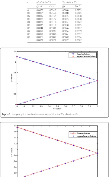
Table 1 The error analysis ofU,Vatx= 0.5
r U(x;r) att= 0.5 V(x;r) att= 0.5 E(x;r) E(x;r) E(x;r) E(x;r)
0 0.0000 0.0147 0.0000 0.0153
0.1 0.0007 0.0140 0.0008 0.0145
0.2 0.0015 0.0132 0.0015 0.0138
0.3 0.0022 0.0125 0.0023 0.0130
0.4 0.0029 0.0118 0.0031 0.0122
0.5 0.0037 0.0110 0.0038 0.0115
0.6 0.0044 0.0103 0.0046 0.0107
0.7 0.0051 0.0096 0.0054 0.0099
0.8 0.0059 0.0088 0.0061 0.0092
0.9 0.0066 0.0081 0.0069 0.0084
1 0.0073 0.0073 0.0077 0.0077
Figure 1Comparing the exact and approximate solutions ofUanduatx= 0.5
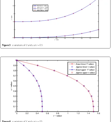
Figure 3 xvariations ofUanduatr= 0.5
Figure 4 xvariations ofVandvatr= 0.5
then Eqs. (9) to (12) can be written in the form
⎧ ⎨ ⎩
u(x;r) = 1 +x2+ex+x
0(x–t)(u(t;r) +v(t;r))dt, u(x;r) = 1 +x2+ex+x
0(x–t)(u(t;r) +v(t;r))dt,
⎧ ⎨ ⎩
v(x;r) = 3 – 3ex+0x(x–t)(u(t;r) –v(t;r))dt, v(x;r) = 3 – 3ex+x
0(x–t)(u(t;r) –v(t;r))dt,
then the system is subject to the triangular fuzzy initial conditions (Definition 7), ul,u(x;r) = [0, 1, 2],vl,u(x;r) = [0, 1, 2], 0≤r≤1. The exact solutions of this illustration is given by
Now, we begin with the primal approximation
u0= –1 +ex+r+· · ·, u0= 1 +ex–r+· · · and
v0= 3 – 3ex–r+· · ·, v
0= 2 –r–x3+· · ·,
and using the above iteration formula, we obtain the successive iterations by using Math-ematica Package10.0.
Error analysis The absolute errors are computed as
E(x;r) =U(x;r) –u(x;r), E(x;r) =U(x;r) –u(x;r) and E(x;r) =V(x;r) –v(x;r), E(x;r) =V(x;r) –v(x;r).
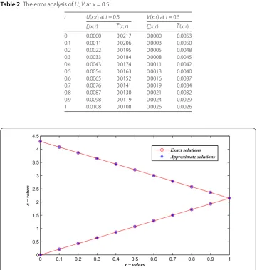
Table 2 The error analysis ofU,Vatx= 0.5
r U(x;r) att= 0.5 V(x;r) att= 0.5 E(x;r) E(x;r) E(x;r) E(x;r)
0 0.0000 0.0217 0.0000 0.0053
0.1 0.0011 0.0206 0.0003 0.0050
0.2 0.0022 0.0195 0.0005 0.0048
0.3 0.0033 0.0184 0.0008 0.0045
0.4 0.0043 0.0174 0.0011 0.0042
0.5 0.0054 0.0163 0.0013 0.0040
0.6 0.0065 0.0152 0.0016 0.0037
0.7 0.0076 0.0141 0.0019 0.0034
0.8 0.0087 0.0130 0.0021 0.0032
0.9 0.0098 0.0119 0.0024 0.0029
1 0.0108 0.0108 0.0026 0.0026
Figure 6Comparing the exact and approximate solutions ofVandvatx= 0.5
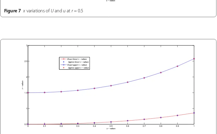
Figure 7 xvariations ofUanduatr= 0.5
The numerical results of the obtained approximate solutions are compared with the exact solutions for differentr-values and errors are presented in Table2. Moreover, exact and approximate solutions are shown graphically in Figs.5and6, thex-variation is also displayed in Figs.7and8. It is clear that we obtain the minimum rate of computation and also get the high accuracy of the result.
6 Conclusion
Recently, many computer programs and techniques have been highly developed for these types of problems, but their scientific discipline basis is for a great deal insufficiently ap-preciated, and the proposed technique is well known as regards the accurate effect of the tomography results. In this research, He’s variational iteration technique is successfully ap-plied on demonstrating results of the Volterra fuzzy integro-differential systems. Utilizing this technique is to quickly lead to the exact result within the minimum rate of iterations and is a very effective tool for evaluating the solutions. The illustrative approaches are tested by the variational iteration technique (by usingMathematica Package10.0).
Acknowledgements
This research was supported by “DST-PURSE-II”. The authors would like to express their sincere thanks to the associate editors and the anonymous reviewers for their constructive comments and valuable suggestions, which have improved the quality of the manuscript.
Funding
Not applicable.
Availability of data and materials
Not applicable.
Competing interests
The authors declare that they have no competing interests.
Authors’ contributions
All authors contributed extensively in the development and completion of this article. Both authors read and approved the final manuscript.
Publisher’s Note
Springer Nature remains neutral with regard to jurisdictional claims in published maps and institutional affiliations.
Received: 6 June 2018 Accepted: 1 October 2018 References
1. Bani Issa, M.S., Hamoud, A.A., Ghadle, K.P., Giniswamy: Hybrid method for solving nonlinear Volterra–Fredholm integro-differential equations. J. Math. Comput. Sci.7(4), 625–641 (2017)
2. Bede, B., Stefanini, L.: Generalized differentiability of fuzzy-valued functions. Fuzzy Sets Syst.230, 119–141 (2013) 3. Dehghan, M., Manafian, J., Saadatmandi, A.: Solving nonlinear fractional partial differential equations using the
homotopy analysis method. Numer. Methods Partial Differ. Equ.26, 448–479 (2010)
4. Dubois, D., Prade, H.: Towards fuzzy differential calculus part 3: differentiation. Fuzzy Sets Syst.8, 225–233 (1982) 5. Ganjiani, M.: Solution of nonlinear fractional differential equations using homotopy analysis method. Appl. Math.
Model.34, 1634–1641 (2010)
6. Ghadle, K.P., Hamoud, A.A.: Study of the approximate solution of fuzzy Volterra–Fredholm integral equations by using (ADM). Elixir Appl. Math.98, 42567–42573 (2016)
7. Ghaneai, H., Hosseini, M.M.: Variational iteration method with auxiliary parameter for solving wave-like and heat-like equations in large domains. Comput. Math. Appl.69(5), 363–373 (2015)
8. Gulsu, M., Sezer, M.: A Taylor collocation method for the approximate solution of general linear Fredholm–Volterra integro-difference equations with mixed argument. Int. J. Comput. Math.175, 675–690 (2006)
9. Hamoud, A.A., Ghadle, K.P.: On the numerical solution of nonlinear Volterra–Fredholm integral equations by variational iteration method. Int. J. Adv. Sci. Tech. Res.3, 45–51 (2016)
10. Hamoud, A.A., Ghadle, K.P.: Modified Adomian decomposition method for solving fuzzy Volterra–Fredholm integral equations. J. Indian Math. Soc.85(1–2), 52–69 (2018)
11. Hamoud, A.A., Ghadle, K.P., Bani Issa, M.S., Giniswamy: Existence and uniqueness theorems for fractional Volterra–Fredholm integro-differential equations. Int. J. Appl. Math.31(3), 333–348 (2018)
13. He, J.H., Wu, G.C., Austin, F.: The variational iteration method which should be followed. Nonlinear Sci. Lett. A, Math. Phys. Mech.1, 1–30 (2010)
14. Inokuti, M., et al.: General use of the Lagrange multiplier in non-linear mathematical physics. In: Nemat-Nasser, S. (ed.) Variational Method in the Mechanics of Solids, pp. 156–162. Pergamon, Oxford (1978)
15. Jafarzadeh, Y., Keramati, B.: Numerical method for a system of integro-differential equations by Lagrange interpolation. Asian-Eur. J. Math.9(3), 1–6 (2016)
16. Jaradat, H.M., Jaradat, I., Alquran, M., Jaradat, M.M.M., Mustafa, Z., Abohassan, K., Abdelkarim, R.: Approximate solutions to the generalized time-fractional Ito system. Ital. J. Pure Appl. Math.37, 699–710 (2017)
17. Karamete, A., Sezer, M.: A Taylor collocation method for the solution of linear integro-differential equations. Int. J. Comput. Math.79, 987–1000 (2002)
18. Khodadadi, E., Çelik, E.: The variational iteration method for fuzzy fractional differential equations with uncertainty. Fixed Point Theory Appl.2013, 13 (2013)
19. Mathankumar, S., Narayanamoorthy, S.: Vaguenesses determinations of hybrid differential equations. Int. J. Pure Appl. Math.117(13), 333–341 (2017)
20. Narayanamoorthy, S., Murugan, K.: A numerical algorithm and a variational iteration technique for solving higher order fuzzy integro-differential equations. Fundam. Inform.133(4), 421–431 (2014)
21. Odibat, Z.M.: A study on the convergence of variational iteration method. Math. Comput. Model.51, 1181–1192 (2010)
22. Qiu, D., Lu, C.X., Zhang, W., Lan, Y.Y.: Algebraic properties and topological properties of the quotient space of fuzzy numbers based on Mareš equivalence relation. Fuzzy Sets Syst.245, 63–82 (2014)
23. Stefanini, L.: A generalization of Hukuhara difference and division for interval and fuzzy arithmetic. Fuzzy Sets Syst.
161, 1564–1584 (2010)