Forward Modeling and validation of a new formulation to compute self potential signals associated with ground water flow

www.hydrol-earth-syst-sci.net/11/1661/2007/ © Author(s) 2007. This work is licensed under a Creative Commons License.

Earth System

Sciences

Forward Modeling and validation of a new formulation to compute

self-potential signals associated with ground water flow

A. Bol`eve1,3, A. Revil1,2, F. Janod3, J. L. Mattiuzzo3, and A. Jardani2,4

1_{CNRS- LGIT (UMR 5559), University of Savoie, Equipe Volcan, Chamb´ery, France}

2_{Colorado School of Mines, Dept. of Geophysics, 1500 Illinois street, Golden, CO, 80401, USA} 3_{SOBESOL, Savoie Technolac, BP 230, F-73375 Le Bourget du Lac Cedex, France}

4_{CNRS, University of Rouen, D´epartement de G´eologie, Rouen, France}

Received: 4 May 2007 – Published in Hydrol. Earth Syst. Sci. Discuss.: 8 June 2007 Revised: 26 September 2007 – Accepted: 9 October 2007 – Published: 16 October 2007

Abstract. The classical formulation of the coupled hydro-electrical flow in porous media is based on a linear formula-tion of two coupled constitutive equaformula-tions for the electrical current density and the seepage velocity of the water phase and obeying Onsager’s reciprocity. This formulation shows that the streaming current density is controlled by the gra-dient of the fluid pressure of the water phase and a stream-ing current couplstream-ing coefficient that depends on the so-called zeta potential. Recently a new formulation has been intro-duced in which the streaming current density is directly con-nected to the seepage velocity of the water phase and to the excess of electrical charge per unit pore volume in the porous material. The advantages of this formulation are numerous. First this new formulation is more intuitive not only in terms of establishing a constitutive equation for the generalized Ohm’s law but also in specifying boundary conditions for the influence of the flow field upon the streaming potential. With the new formulation, the streaming potential coupling coef-ficient shows a decrease of its magnitude with permeability in agreement with published results. The new formulation has been extended in the inertial laminar flow regime and to unsaturated conditions with applications to the vadose zone. This formulation is suitable to model self-potential signals in the field. We investigate infiltration of water from an agricul-tural ditch, vertical infiltration of water into a sinkhole, and preferential horizontal flow of ground water in a paleochan-nel. For the three cases reported in the present study, a good match is obtained between finite element simulations per-formed and field observations. Thus, this formulation could be useful for the inverse mapping of the geometry of ground-water flow from self-potential field measurements.

Correspondence to: A. Revil

([email protected])

1 Introduction

Self-potential signals are electrical fields passively mea-sured at the ground surface of the Earth or in boreholes using non-polarizing electrodes (e.g., Nourbehecht, 1963; Ogilvy, 1967). Once filtered to remove anthropic signals and telluric currents, the residual self-potential signals can be associated with polarization mechanisms occurring in the ground (e.g., Nourbehecht, 1963; Bogoslovsky, and Ogilvy, 1972, 1973; Kilty and Lange, 1991; Maineult et al., 2005). One of the main polarization phenomena occurring in the ground is ground water flow (e.g., Ogilvy et al., 1969; Bo-goslovsky, and Ogilvy, 1972; Sill, 1983; Aubert and Atan-gana, 1996) with a number of applications in hydrogeology (Bogoslovsky, and Ogilvy, 1972, 1973; Kilty and Lange, 1991; Maineult et al., 2005; Wishart et al., 2006), in the study of landslides in combination with electrical resistiv-ity tomography (Lapenna et al., 2003, 2005; Perrone et al., 2004; Colangelo et al., 2006), the study of leakages through dams (e.g., Bogoslovsky, and Ogilvy, 1973; Gex, 1980), and in the study in the geohydrology of volcanoes (e.g., Aubert et al., 2000; Aizawa, 2004; Finizola et al., 2004; Ishido, 2004; Bedrosian et al., 2007). The electrical field associated with the flow of the ground water is called the streaming potential (e.g., Ernstson and Scherer, 1986; Wishart et al., 2006) and is due to the drag of the net (excess) electrical charge of the pore water by the flow of the ground water (e.g., Ishido and Mizutani, 1981).

Another contribution to self-potential signals over contam-inated ground water is the biogeobattery model developed by Arora et al. (2007) and Linde and Revil (2007) based on the field and laboratory observations reported by Naudet et al. (2003, 2004) and Naudet and Revil (2005). This contri-bution will not be discussed in this paper.

-6 -4 -2

-3.2 -2.8 -2.4 -2 -1.6 -1.2 -0.8 -0.4 0 0.2

Self-potential (mV)

Datum

Depth (m)

Unconfined aquifer Vadose zone P

M

Current source generator

u

V

Ref Observation point

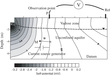
Fig. 1. Sketch of the flow of the ground water from a ditch in an

un-confined aquifer and the resulting self-potential distribution. Each point of the ground M where is a net flow of the ground water wa-ter can be represented as a source generator of electrical currents. Each elementary source of current is responsible for an electrical field obtain by solving the Poisson equation. The sum of these elec-trical fields is sampled at the ground surface using a pair of non-polarizing electrodes. One of these electrodes is used as a reference while the other is used to measure, at different stations, the value of the electrical potential (called the self-potential) with respect to the reference.

instrumental in the improvement of the self-potential method for applications in hydrogeophysics (see Perrier and Morat, 2000; Suski et al., 2007 and references therein). One of the first numerical computation of streaming potentials due to ground water flow was due to Sill (1983) who used a 2-D finite-difference code. Sill (1983) used a set of two coupled constitutive equations for the electrical current density and the seepage velocity. These constitutive equations were cou-pled with two continuity equations for the electrical charge and the mass of the pore water. In this classical formula-tion, the source current density is related to the gradient of the pore fluid pressure and to a streaming current coupling coefficient that depends on the so-called zeta-potential, a key electrochemical property of the electrical double layer coat-ing the surface of minerals in contact with water (e.g., Ishido and Mizutani, 1981; Leroy and Revil, 2004). Later, Wurm-stich et al. (1991) performed numerical simulations of the self-potential response associated with the flow of the pore water in a dam.

The classical formulation of Sill (1983) was used by many authors in the two last decades (e.g., Fournier, 1989; Birch, 1993; Santos et al., 2002; Revil et al., 2003, 2004; Suski et al., 2007). While it has proven to be useful, this formula-tion has however several drawbacks. Intuitively, one would expect that self-potential signals would be more related to the seepage velocity than to the pore fluid pressure. This is especially true in unsaturated conditions for which only the existence of a net velocity of the water phase can be

responsi-ble for a net current source density. In addition, the classical formulation does not explain the observed dependence of the streaming potential with the permeability reported by Jou-niaux and Pozzi (1995) almong others. It was also difficult to extend the classical formulation to unsaturated conditions (Jiang et al., 1998; Perrier and Morat, 2000; Guichet et al., 2003; Revil and Cerepi, 2004) despite the fact that there is a strong interest in using self-potential signals to study the in-filtration of water through the vadose zone (e.g., Lachassagne and Aubert, 1989).

Recently, a new formulation has been developed by Re-vil and Leroy (2004) and ReRe-vil et al. (2005a). This formu-lation was generalized to a multi-component electrolyte by Revil and Linde (2006), who also modeled the other con-tributions to self-potential signals for a porous material of arbitrary texture and an electrolyte of arbitrary composition. The formulation of Revil et al. (2005a) was initially devel-oped to determine the streaming potential coupling coeffi-cient of clay-rocks. However, it seems to work fairly well for any type of porous materials. This formulation connects the streaming current density directly to the seepage velocity and to the excess of charge per unit pore volume. This excess of charge corresponds to the excess of charge due to the dif-fuse layer counterbalancing the surface charge density of the surface of the minerals including the ions sorbed in the so-called Stern layer. Unlike the classical formulation, the new one is easily extendable to unsaturated conditions (see Linde et al., 2007, Revil et al., 2007) and to non-viscous laminar flow conditions at high Reynolds numbers (see Crespy et al., 2007; Bol`eve et al., 2007). In both cases, an excellent agree-ment was obtained between the theory and the experiagree-mental data. However, so far this formulation has been tested only in the laboratory and not yet on field data.

In the present paper, we test the new formulation of Revil and Linde (2006) to determine numerically, using the com-mercial finite element code Comsol Multiphysics 3.3 (Com-sol, 2007), the self-potential response in the field associated with ground water flow. Three recently published field cases are reanalyzed with the new formulation to see its potential to model field data. The challenge will be to invert self-potential signals directly in terms of ground water flow in future studies.

2 Description of the new formulation

2.1 Saturated case

self-potential signals that is related to the flow of the ground water (Fig. 1).

We consider a water-saturated mediums isotropic but pos-sibly heterogeneous. In the classical formulation of the streaming potential, electrical and hydraulic processes are coupled through the following two constitutive equations op-erating at the scale of a representative elementary volume of the porous material (e.g., Ishido and Mizutani, 1981; Morgan et al., 1989; Jouniaux and Pozzi, 1995; Revil et al., 1999a, b):

j = −σ∇ϕ−L(∇p−ρfg), (1)

u= −L∇ϕ− k

ηf

(∇p−ρfg), (2)

C=

_∂ϕ

∂p

j=0

= −L

σ, (3)

wherej is the electrical current density (in A m−2),uis the seepage velocity (in m s−1)(Darcy velocity), −∇ϕ is the electrical field in the quasi-static limit of the Maxwell equa-tions (in V m−1),p is the pore fluid pressure (in Pa), g is the gravity acceleration vector (in m s−2_{), σ andk are the} electrical conductivity (in S m−1_{)and intrinsic permeability} (in m2)of the porous medium, respectively,ρf andηf are

the mass density (in kg m−3_{)and the dynamic shear} viscos-ity (in Pa s) of the pore water, andLis both the streaming current coupling coefficient and the electroosmotic coupling coefficient (in m2V−1s−1), andC(in V Pa−1)is the stream-ing potential couplstream-ing coefficient. The symmetry of the cou-pling terms in Eqs. (1) and (2) is known as the Onsager’s reciprocity (Onsager, 1931). It holds only in the vicinity of thermodynamic equilibrium to ensure the positiveness of the dissipation function (Onsager, 1931).

The hydroelectrical coupling terms existing in Eqs. (1) and (2) is said to be electrokinetic, i.e., it is due to a relative dis-placement between the charged mineral surface and its as-sociated electrical double (or triple) layer (e.g., Ishido and Mizutani, 1981; Morgan et al., 1989). The streaming current density−L(∇p−ρfg)is due to the drag of the electrical

excess charge contained in the electrical diffuse layer while the term−L∇ϕ in Eq. (2) is due to the viscous drag of the pore water associated with the displacement of the excess of electrical charge in an electrical field. In the classical for-mulation described above, the streaming potential coupling coefficient is related to the zeta potential (a key electrochem-ical property of the electrelectrochem-ical double layer coating the surface of the minerals, e.g., Kosmulski and Dahlsten, 2006) by the so-called Helmholtz-Smoluchowski equation (see Ishido and Mizutani, 1981; Morgan et al., 1989). In situations where the surface conductivity of the grains can be neglected, the Helmholtz-Smoluchowski equation predicts that the stream-ing potential couplstream-ing coefficient does not depend on the tex-ture of the porous material.

The alternative formulation to Eq. (1) is (Revil and Leroy, 2004, Revil et al., 2005a, and Revil and Linde, 2006),

j =σE− ¯QVu, (4)

whereE=−∇ϕis the electrical field andQ¯V is the excess of

charge (of the diffuse layer) per unit pore volume (in C m−3_). Equation (4) can be derived by upscaling the Nernst-Planck equation (Revil and Linde, 2006).

An equation for the seepage velocity including an elec-troosmotic contribution can also be developed based on the new formulation introduced by Revil and Linde (2006). However, this contribution can be safely neglected if the only component of the electrical field is that produced through the electrokinetic coupling (e.g., Sill, 1983). Using this approxi-mation, we recover the Darcy constitutive equation:

u= −K∇H, (5)

where K is the hydraulic conductivity (in m s−1) and

H=δp/ρfgis the change in hydraulic head (above or below

the hydrostatic initial distributionH0). Combining Eqs. (3), (4), and (5), the streaming potential coupling coefficient in the new formulation is given byC= − ¯QVk/(σ ηf)(see

Re-vil and Leroy, 2004, and ReRe-vil et al., 2005a). We can also in-troduce a streaming potential coupling coefficient relative to the hydraulic headC0=∂ϕ/∂H= − ¯QVK/σ. These

relation-ships show a connection between the coupling coefficientsC

orC’ and the permeabilitykor the hydraulic conductivityK. If we use these relationships, the two formulations, Eq. (2) and (4) are strictly equivalent in the saturated case. The only difference lies in the relationship between the streaming cou-pling coefficient and the microstructure. With the classical formulation, the use of the Helmholtz-Smoluchowski equa-tion predicts that the streaming potential coupling coefficient does not depend on the microstructure. At the opposite, the new formulation predicts that the streaming potential cou-pling coefficient depends on the microstructure in agreement with experimental data (see Jouniaux and Pozzi, 1995).

The constitutive equations, Eqs. (4) and (5), are completed by two continuity equations for the electrical charge and the mass of the pore water, respectively. The continuity equation for the mass of the pore fluid is:

S∂H

∂t = ∇ ·(K∇H ), (6)

whereS is the poroelastic storage coefficient (expressed in m−1_{)assuming that the material behaves as an} electro-poro-elastic medium. The continuity equation for the electrical charge is,

∇ ·j =0, (7)

which means that the current density is conservative in the quasi-static limit of the Maxwell equations. Combining Eqs. (4) and (7) results in a Poisson equation with a source term that depends only on the seepage velocity in the ground:

E9 E1 E36 E41 E10 E18 E19 E27 E28 E35

-2 0 2 4 6

-2 0 2 4 6 8 10 B0 B1 B2 B4 B'4 B'6 W2 W1 A0 A1 A2 A3 A4 A6 C0 C1 C2 C4 C'4 C'6

x, Distance (m)

Ditch

y

, Distance (m)

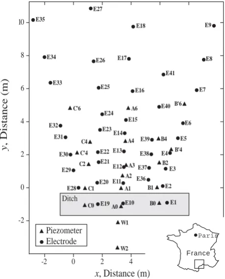
Piezometer Electrode E2 E3 E4 E5 E6 E7 E8 E37 E38 E39 E40 E11 E12 E13 E14 E15 E16 E17 E20 E21 E22 E23 E24 E25 E26 E29 E30 E31 E32 E33 E34 8 France Paris

Fig. 2. Top view the test site for the infiltration experiment showing

the position of the electrodes and the piezometers. The reference electrode is located 100 m away from the ditch.

where=is the volumetric current source density (in A m−3)

given by,

= = ¯QV∇ ·u+ ∇ ¯QV ·u, (9)

In steady state conditions,∇ ·u=0 and therefore we have,

= = ∇ ¯QV ·u, (10)

i.e., the only source term in steady-state conditions. The shape of the electrical potential streamlines is also influenced by the distribution of the electrical conductivity distribution existing in the ground.

2.2 Unsaturated case

For unsaturated conditions, the hydraulic problem can be solved using the Richards equation with the van Genuchten parametrization for the capillary pressure and the relative permeability of the water phase. The governing equation for the flow of the water phase is (Richards, 1931),

[Ce+SeS] ∂H

∂t + ∇ ·[−K∇(H +z)]=0, (11)

wherezis the elevation above a datum,H (m) is the pres-sure head, Ce denotes the specific moisture capacity (in

m−1) defined by Ce=∂θ/∂H where θ is the water

con-tent (dimensionless), Se is the effective saturation, which

is related to the relative saturation of the water phase by

Se=(Sw−Swr)/(1−Swr) whereSwr is the residual saturation

of the wetting phase andSw is the relative saturation of the

water phase in the pore space of the porous medium (θ=Swφ

whereφrepresents the total connected porosity of the mate-rial),S is the storage coefficient (m−1), andt is time. The hydraulic conductivity is related to the relative permeabil-itykr and to the hydraulic conductivity at saturationKs by K=krKs.

With the van Genuchten parametrization, we consider the soil as being saturated when the fluid pressure reaches the atmospheric pressure (H=0). The effective saturation, the specific moisture capacity, the relative permeability, and the water content are defined by,

Se=

1/

1+ |αH|nm

, H <0

1, H≥0 (12)

Ce= 



 αm

1−m(φ−θr) S

1

m e

1−S

1

m e

m

, H <0 0, H≥0

(13)

kr = 





S_eL

1−

1−S

1

m e

m2

, H <0 1, H ≥0

(14)

θ=

θr+Se(φ−θr) , H <0

φ, H ≥0 (15)

respectively and where θr is the residual water content

(θr=Swrφ), and α, n, m, and L are parameters that

char-acterize the porous material with usually m=1–1/n (van Genuchten, 1980; Mualem, 1986).

The total electrical current density (generalized Ohm’s law) is given by (Linde et al., 2007; Revil et al., 2007),

j =σ (Sw)E+ ¯

QV SW

u, (16)

whereu= −(krKs/ηf)∇H (andu=0 whenSw→Swr). The

continuity equation is ∇ ·j=0. The effect of the relative saturation upon the electrical conductivity can be determined using second Archie’s law (Archie, 1942). Archie’s second law is valid only when surface conductivity can be neglected. When the influence of surface conductivity cannot be ne-glected, more elaborate models (e.g., Waxman and Smits, 1968; Revil et al., 1998; Revil et al., 2002a) can be used instead.

3 Infiltration test from a ditch

part France (Fig. 2) on the plain of the H´erault River. Eigh-teen piezometers were installed to a depth of 4 m on one side of the ditch (Fig. 2). The ditch itself was 0.8 m deep, 1.5 m wide, and 10 m long (Fig. 2a). The self-potential signals were monitored using a network of 41 non-polarising Pb/PbCl2 electrodes (PMS9000 from SDEC) buried in the ground near the ground surface and a Keythley 2701 Multichannel volt-meter (with 80 channels). Suski et al. (2006) performed also an electrical resistivity tomography (ERT) along a section perpendicular to the ditch. The ERT allows to image the re-sistivity of the ground to a depth of 5 m (the acquisition was done with a set of 64 electrodes using the Wenner-αarray and a spacing of 0.5 m between the electrodes). This ERT indicates that the resistivity of the soil was roughly equal to 20 Ohm m except for the first 50 cm where the resistivity was

∼100 Ohm m.

The piezometers show that the water table was initially lo-cated at a constant depth of 2 m below the ground surface. During the experiment, 14 m3of fresh water was injected in the ditch. The electrical conductivity of the injected water was 0.068 S m−1at 20◦C. The infiltration experiment can be divided into three phases. Phase I corresponds to the increase of the water level with time in the ditch until a hydraulic head (measured from the bottom of the ditch) of 0.35 m was reached. The duration of this phase is≈12 min. In Phase II, the hydraulic head was maintained constant for 3 h. At the beginning of phase III, we stopped the injection of wa-ter. This third phase corresponds therefore to the relaxation of the phreatic surface over time. The monitoring network of electrodes was activated at 07:28 LT (Local Time). The infiltration of the water in the ditch started at 08:48 LT (be-ginning of Phase I). The hydraulic and electrical responses were monitored during 6 h and 20 min.

Laboratory experiments of the streaming potential cou-pling coefficients (see Suski et al., 2006) yields C’=– 5.8±1.1 mV m−1. The measurement was performed using the conductivity of the water injected into the ditch. All the hydrogeological material properties used in the following fi-nite element numerical simulation are reported in Table 1. This table is using the hydrogeological model of Dag`es et al. (2007)1, which uses only hydrogeological inputs. The electrical conductivity of each soil layer and its streaming po-tential coupling coefficient are reported in Table 2 from the experimental and field data reported by Suski et al. (2006).

A 2-D numerical simulation was performed with a com-mercial finite element code (Comsol Multiphysics 3.3) along a cross-section perpendicular to the ditch (Fig. 3). Because of the symmetry of the problem with an axis of symmetry corresponding to the ditch, only one side of the ditch is mod-eled. We use the full formulation including capillary effects 1_{Dag`es, C., Voltz, M., and Ackerer, P.: Parameterization and}

evaluation of the three-dimensional modelling approach to water table recharge from seepage losses in a ditch, Adv. Ground Water, submitted, 2007.

0.4 0.5 0.6 0.7 0.8 0.9 1 Saturation

D

e

pth (m)

Distance (m)

-0

-1

-2

-3

-- -- -- -- --

-0 1 2 3 4 5

Fig. 3. Snapshot of the relative water saturation during the

infiltra-tion experiment. The saturainfiltra-tion is determined using the finite ele-ment code Comsol Multiphysics 3.3. The arrows show the seepage velocities.

D

epth (m)

Distance (m)

-0

-1

-2

-- -- -- -- --

-0 1 2 3 4 5

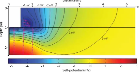
Self-potential (mV)

-5 -4 -3 -2 -1 0 1 2 3

0 mV -1 mV

-2 mV -3 mV -4 mV

Fig. 4. Snapshot of the self-potential signal (in mV) along a

verti-cal cross-section perpendicular to the ditch. A negative anomaly is observed in the vicinity of the ditch.

in the vadose zone and therefore the influence of the capil-lary fringes using these material properties (see Sect. 2.2). Before the beginning of the injection of water in the ditch, the water table is located at a depth of 2 m with a stable cap-illarity fringe determined according to the van Genuchten pa-rameters given in Table 1. Inside the ditch, we imposed a hy-draulic head that varies over time according to the water level observing during the infiltration experiment in Stage I to III (see Suski et al., 2006). For electrical problem, we use in-sulating boundary conditionn.j=0 at the ground surface and at the symmetry plane (atx=0) andϕ→0 at infinity, where, ideally, the reference electrode is supposed to be.

Table 1. Porosity,φ; residual water contentθr, van Genuchten parametersnandα(we considerL=0.5 andm=1–1/n), hydraulic conductivity at saturationKs, anisotropy coefficient for the hydraulic conductivity at saturation for the four soil horizons in the ditch infiltration experiment (parameters taken from the hydrogeological computation performed by Dag`es et al., 20071).

Layer Depths φ θr n α Ks Anisotropy

(m) (mm−1) (m s−1) coefficient

1 0–0.9 0.37 5.1×10−5 1.296 0.01360 1.11×10−4 1.5 2 0.9–2.2 0.33 5.7×10−4 1.572 0.00240 3.05×10−5 1.0 3 2.2–3.5 0.31 5.5×10−4 1.279 0.00520 5.00×10−5 2.5 4 3.5–6.0 0.33 5.7×10−4 1.572 0.00240 3.05×10−5 1.0

Table 2. Electrical conductivity and streaming current coupling

co-efficient for all soil layers involved in the model of the infiltration experiment.

Soil layers σ(S m−1) Q¯V (in C m−3)

1 0.01×S2_w(1) 0.33 2 0.01×S2_w(1) 1.21

3 0.05 0.74

4 0.05 1.21

(1)_{Using second Archie’s law (Archie, 1942).}

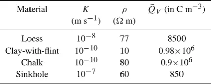
Table 3. Material properties used for the numerical simulation for

the sinkhole case study.

Material K ρ Q¯V (in C m−3)

(m s−1) (m)

Loess 10−8 77 8500

Clay-with-flint 10−10 10 0.98×106

Chalk 10−10 80 0.9×106

Sinkhole 10−7 60 850

4 Infiltration through sinkholes

The second test site discussed in this paper is located in Nor-mandy (Fig. 6). It was recently investigated by Jardani et al. (2006a, b) (see also recently Jardani et al., 2007, for a joint inversion of EM34 and self-potential data at the same site). Jardani et al. (2006a) performed 225 self-potential measure-ments in March 2005 with two Cu/CuSO4electrodes to map the self-potential anomalies in a field in which several sink-holes are clustered along a north-south trend (Fig. 6). They used a Metrix MX20 voltmeter with a sensitivity of 0.1 mV and an internal impedance of 100 MOhm. The standard devi-ation on the measurements was smaller than one millivolt be-cause of the excellent contact between the electrodes and the ground. The self-potential map shows a set of well-localized

-5 -4 -3 -2 -1 0 1

0 2 4 6 8 10 12

Sel

f po

te

nt

ia

l (i

n

mV)

Distance to the ditch (in m)

Fig. 5. Comparison between the measured self-potential signals

(the filled triangles)along profile P3 (see Fig. 1) and the computed self-potential profile (the plain line). The error bars denote the stan-dard deviation on the measurements.

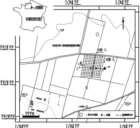
negative self-potential anomalies associated with the direc-tion along which the sinkholes are clustered. In this paper, we investigate only the profile AB (see location on Fig. 6) along which a high-resolution self-potential profile was ob-tained together with a resistivity profile.

P.1

x(m)

y(m) 497000 497300 497600

209400 209600

209200 209800

497000 497300 497600 N

Réf 119 m

116m 116m

100m

Route N115

Le Hameau de la route

A B

Sinkholes Wells SP stations France

Paris

Fig. 6. The test site is located in Normandy, in the North-West of

France, near the city of Rouen. The small filled circles indicate the position of the self-potential (SP) stations, Ref represents the reference station for the self-potential measurements, and P1 corre-sponds to the trace of the electrical resistivity survey. Note that the sinkholes are organized along a North-South trend.

0

-4

-8

-12

Distance (in meters)

-10 0 10 20 30 40 50 60 70 80 90 100 110

Sinkhole Clay-with-flint

Chalk Loess

∂Ω1 ∂Ω2 ∂Ω1

∂Ω3

∂Ω4

∂Ω3

Depth (in meters)

Fig. 7. Geometrical model used for the finite element calculation.

The geometry of the interface between the loess and the clay with flint formation is determined from the resistivity tomogram. The material properties used for the calculations are discussed in the main text. The reference electrode is assumed to be located in the upper left-hand side corner of the profile.

we fixed the flux equal to the infiltration capacity of the sink-hole (10−7m2s−1, that is 3 m year−1)because of the ob-served runoff of water in sinkholes in this area (Jardani et al., 2006a). The geometry of the system is shown on Fig. 7. At the upper boundaryδ1, the hydraulic flux is set equal to the rain rate (0.6 m yr−1_{), opposite vertical sides of the} system are characterized by impermeable boundary condi-tionsn.u=0 (because the infiltration is mainly vertical). At the lower boundaryδ4, we fixed the flux for the ground water equal to the exfiltration capacity of the sinkhole. The lower boundaryδ3 is considered to be impermeable. For the electrical problem, we use the insulating boundary condi-tion,n.j=0 at the interface between the atmosphere and the

-10 0 10 20 30 40 50 60 70 80 90 100 110

0

-5

-10

-15

Distance (m)

D

e

pth (m)

-30 -20 -10 0 10 20 30

Self potential (mV)

Fig. 8. 2-D finite element simulation of the self-potential (expressed

in mV) along the resistivity profile AB (see location on Fig. 5). The reference electrode is assumed to be located in the upper left-hand side corner of the profile.

-4040 -3030 -2020 -1010 0 10 10 20 20

-4040 -2020 0 2020 4040 6060 8080 100100

S

el

f potf

p

o

te

ntn

ti

al

(m (

m

V

)

di distancnce (m (m)

Fig. 9. The reference electrode is assumed to be located in the

up-per left-hand side corner of the profile. The error bar (±1 mV) is determined from the standard deviation determined in the field for the self-potential measurements.

ground. The reference electrode for the self-potential sig-nal is located atx=−10 m at the ground surface. In order to match the observed data, one should choose the same refer-ence in the numerical modeling.

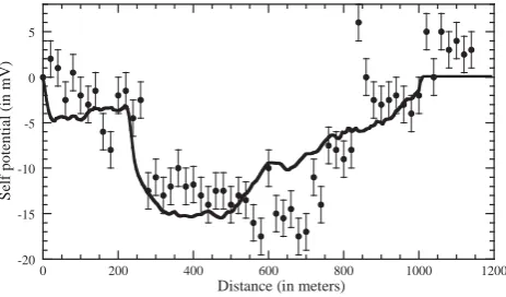
The result of the numerical simulations is shown on Fig. 8. A comparison between the self-potential data and the simu-lated self-potential data is shown on Fig. 9 along the pro-file AB. Despite some minor variations between the model and the measured data (likely due to the two-dimensional ge-ometry used in the model while the real gege-ometry is three-dimensional), the model is able to capture the shape of the self-potential anomalies.

5 Flow in a Paleochannel

VACCARES POND

MAP of MEJANES

PALEO-CHANNEL

500 m

FRANCE

Vaccarès pond

Camargues

a.

b.

b. c.

c.

C

D

Fig. 10. Localization of the test site in Camargue, in the delta of the

Rhˆone river. The profile CD corresponds to the resistivity profile shown on Fig. 10. The yellow plain lines represent self-potential profiles described in Revil et al. (2005b).

Buried channel

Unit electrode spacing 5 meters

Electrical resistivity (Ohm m)

Depth (m)

0 5 10 15 20 25

0.5 1 5 10 40

C D

Substratum

Paleo-channel Substratum

-20 -15 -10 -5 0 5

0 200 400 600 800 1000

Negative self-potential anomaly

Self-potential (in mV)

Silt and sand Claystone S6

Fig. 11. Electrical resistivity tomography and self-potential

anomaly along a cross-section perpendicular to the paleochannel. We observe a negative self-potential anomaly above the position of the buried paleochannel. According to Revil et al. (2005b), the contrast of resistivity between the plaeochannel and the surround-ing sediment is due to a strong contrast of resistivity between the pore water filling the paleochannel and the pore water filling the surrounding sediments.

by fluvial deposits of an ancient channel of the Rhˆone river named the Saint-Ferr´eol Channel. In principle, the salin-ity of the M´ejanes area is high due to saltwater intrusion in the vicinity of the saline pond. The self-potential volt-ages were mapped with two non-polarising Pb/PbCl2 elec-trodes (PMS9000 from SDEC) and a Metrix MX20 voltmeter with a sensitivity of 0.1 mV and an internal impedance of 100 MOhm.

Electrical resistivity tomography indicates that resistivity of the sediment outside the buried paleo-channel is in the range 0.4–1.2(Fig. 11). According to Revil et al. (2005b),

Distance (m)

D

epth (m)

0 100 200 300 400 500 600 700 800 900 0

-5 -10 -15 -20

-25

-14 -12 -10 -8 -6 -4 -2 0 Self-potantial (mV)

-6 mV -8 mV

-12 mV -12 mV

-14 mV -14 mV

-10 mV

Fig. 12. Computation of the self-potential signals (expressed in

mV) inside the paleochannel across a cross-section perpendicular to the paleochannel. The computation is performed using 3-D sim-ulation of the coupled hydroelectric problem in the paleochannel. The reference electrode is assumed to be located in the upper left-hand side corner of the profile. Note that the interface between the paleochannel and the surrounding body is an equipotential.

this implies that the resistivity of the pore water is in the range 0.1– 0.4m in the paleochannel. Therefore, the ground water in the paleochannel is approximately ten time less saline than the pore water contained in the surrounding sediments. Inside the paleo-channel, the streaming potential coupling coefficient is equal to−1.2±0.4 mV m−1based on the range of values for the resistivity of the pore water and laboratory measurements given by Revil et al. (2005b). The magnitude of the streaming potential coupling coefficients in the surrounding sediments is<0.2 mV m−1, so much smaller than inside the paleochannel and will be neglected in the nu-merical simulation.

For the numerical simulations, we use a permeability equal to 10−10m2, a streaming potential coupling coefficient equal to−1.2±0.4 mV m−1_{, and an electrical conductivity equal} to 0.035 S m−1_{for the materials filling the paleochannel. At} the entrance of the paleochannel, we impose a flux equal to 8×10−4m s−1. We assume that the sediment is impermeable outside the paleochannel and we use the continuity of the normal component of the electrical current density through the interface between the paleochannel and the surrounding sediments.

-20 -15 -10 -5 0 5

0 200 400 600 800 1000 1200

S

el

f pot

en

ti

al

(i

n m

V

)

Distance (in meters)

Fig. 13. Comparison between the measured self-potential signals

(reported in Revil et al., 2005b) along a cross-section perpendicu-lar to the paleochannel (the filled circles) and the computed self-potential profile using the finite element code Comsol Multiphysics 3.3. The error bars were determined from the standard deviation determined in the field for the self-potential measurements.

6 Concluding statements

Self-potential signals can be computed directly from the seepage velocity and the excess of charge per unit pore volume of the porous medium. This excess of electrical charge can be determined from the streaming potential cou-pling coefficient at saturation and the hydraulic conductivity through laboratory measurements. In saturated conditions, the macroscopic formulation we used is similar to the clas-sical formulation except that it accounts for the permeability of the formations upon the streaming current density. In ad-dition, the new formulation can be extended to unsaturated conditions and can therefore be used to determine the effect of the capillary fringe, for example, upon the measured self-potential signals. Numerical simulations performed at differ-ent test sites shows that our formulation can be used to rep-resent quantitatively the self-potential signals in field condi-tions. In this regard, the analysis provided in this paper paves the way for future inverse reconstruction of important hydro-logical parameters (permeability, flow velocity, and aquifer geometry) from collocated self-potential and electrical resis-tivity measurements on the ground’s surface or in boreholes. The inversion of self-potential signals is a relatively new field (see Jardani et al., 2006b; Minsley et al., 2007; Mendonc¸a, 2007) with a high number of potential applications in hydro-geology, and especially to pumping tests (Rizzo et al., 2004; Suski et al., 2004; Titov et al., 2005; and Straface et al., 2007) as well as the scale of catchments (Linde et al., 2007). The effect of the heterogeneity of the resistivity and the coupling coefficient will be investigated in a forthcoming work. Acknowledgements. This work was supported by the CNRS (The

French National Research Council), by ANR Projects ERINOH and POLARIS. We thank ANR (Agence Nationale de la Recherche), the French National Program “ECosph`ere Continentale” and INSU-CNRS for their financial supports. The Ph-D Thesis of

A. Bol`eve is supported by SOBESOL and ANRT. We thank Maxwell Meju and an anonymous referee for their constructive comments.

Edited by: C. Hinz

References

Aizawa, K.: A large self-potential anomaly and its changes on the quiet Mt. Fuji, Japan, Geophys. Res. Lett., 31, L05612. doi:10.1029/2004GL019462, 2004.

Archie, G. E.: The electrical resistivity log as an aid in determining some reservoir characteristics, Trans. AIME, 146, 54–61, 1942. Arora T., Linde N., Revil A., and Castermant J.: Non-intrusive

de-termination of the redox potential of contaminant plumes by us-ing the self-potential method, J. Contaminant Hydrol., 92, 274– 292, doi:10.1016/j.jconhyd.2007.01.018, 2007.

Aubert, M., Dana, I. N., Gourgaud, A.: Internal structure of the Merapi summit from self-potential measurements, J. Volcanol. Geotherm. Res., 100(1), 337–343, 2000.

Aubert, M. and Atangana, Q. Y.: Self-potential method in hydroge-ological exploration of volcanic areas, Ground Water, 34, 1010– 1016, 1996.

Bedrosian, P. A., Unsworth, M. J., and Johnston, M. J. S.: Hy-drothermal circulation at Mount St. Helens determined by self-potential measurements, J. Volcanol. Geotherm. Res., 160(1–2), 137–146, 2007.

Birch F. S.: Testing Fournier’s method for finding water table from self-potential, Ground Water, 31, 50–56, 1993.

Bol`eve, A., Crespy, A., Revil, A., Janod, F., and Mattiuzzo, J. L.: Streaming potentials of granular media. Influence of the Dukhin and Reynolds numbers, J. Geophys. Res., 112, B08204, doi:10.1029/2006JB004673, 2007.

Bogoslovsky, V. A. and Ogilvy, A. A.: The study of streaming potentials on fissured media models, Geophys Prospecting, 51, 109–117, 1972.

Bogoslovsky, V. A. and Ogilvy, A. A.: Deformation of natural elec-tric fields near drainage structures, Geophys. Prospecting, 21, 716–723, 1973.

Colangelo, G., Lapenna, V., Perrone, A., et al.: 2D Self-Potential tomographies for studying groundwater flows in the Varco d’Izzo landslide (Basilicata, southern Italy), Engineering Geol-ogy, 88(3–4), 274–286, 2006.

Comsol: http://www.comsol.com/, 2007.

Crespy, A., Bol`eve, A., and Revil, A.: Influence of the Dukhin and Reynolds numbers on the apparent zeta potential of granular me-dia, J. Colloid Interface Sci., 305, 188–194, 2007.

Ernstson, K. and Scherer, H. U.: Self-potential variations with time and their relation to hydrogeologic and meteorological parame-ters, Geophysics, 51, 1967–1977, 1986.

Finizola, A., L´enat, J. F., Macedo, O., Ramos, D., Thouret, J. C., and Sortino, F.: Fluid circulation and structural discontinuities inside Misti volcano (Peru) inferred from self-potential measure-ments, J. Volcanol. Geotherm. Res., 135, 343–360, 2004. Finizola, A., Sortino, S., L´enat, J.-F., Aubert, M., Ripepe, M.,

impli-cations, Bull. Volcanol., 65, 486–504, doi:10.1007/s00445-003-0276-z, 2003.

Fournier, C.: Spontaneous potentials and resistivity surveys applied to hydrogeology in a volcanic area: case history of the Chaˆıne des Puys (Puy-de-Dˆome, France), Geophys. Prospecting, 37, 647– 668, 1989.

Guichet, C., Jouniaux, L., and Pozzi, J.-P.: Streaming potential of a sand column in partial saturation conditions, J. Geophys. Res., 108, 2141–2153, 2003.

Ishido, T. and Mizutani, H.: Experimental and theoretical basis of electrokinetic phenomena in rock-water systems and its applica-tion to geophysics, J. Geophys. Res., 86, 1763–1775, 1981. Ishido, T.: Electrokinetic mechanism for the “W”-shaped

self-potential profile on volcanoes, Geophys. Res. Lett., 31, L15616. doi:10.1029/2004GL020409, 2004.

Jardani, A., Revil, A., Santos, F., Fauchard, C., and Dupont, J. P.: Detection of preferential infiltration pathways in sinkholes using joint inversion of self-potential and EM-34 conductiv-ity data, Geophys. Prospecting, 55, 1–11, doi:10.1111/j.1365-2478.2007.00638.x, 2007.

Jardani A., Dupont, J. P., and Revil, A.: Self-potential signals asso-ciated with preferential ground water flow pathways in sinkholes, J. Geophys. Res., 111, B09204, doi:10.1029/2005JB004231, 2006a.

Jardani, A., Revil, A., and Dupont, J. P.: 3D self-potential tomogra-phy applied to the determination of cavities, Geotomogra-phys. Res. Lett., 33, L13401, doi:10.1029/2006GL026028, 2006b.

Jiang, Y. G., Shan, F. K., Jin, H. M., Zhou, L. W., and Sheng, P.: A method for measuring electrokine tic coefficients of porous media and its potential application in hydrocarbon exploration, Geophys. Res. Lett., 25(10), 1581–1584, 1998.

Jouniaux, L. and Pozzi, J.-P.: Streaming potential and permeability of saturated sandstones under triaxial stress: Consequences for electrotelluric anomalies prior to earthquakes, J. Geophys. Res., 100, 10 197–10 209, 1995.

Kosmulski, M. and Dahlsten, P.: High ionic strength electrokinetics of clay minerals. Colloids and Surfaces A: Physicochem. Eng. Aspects, 291, 212–218, 2006.

Kilty, K. T. and Lange, A. L.: Electrochemistry of natural potential processes in karst. In: Proc 3rd Conf on Hydrogeology, Ecology, Monitoring, and Management of Groundwater in Karst Terranes, 4–6 Dec 1991, Maxwell House, Clarison, Nashville, Tennessee, 163–177, 1991.

Lachassagne, P. and Aubert, M.: Etude des ph´enom`enes de polari-sation spontan´ee (PS) enregistr´ees dans un sol lors de transferts hydriques verticaux, Hydrog´eologie, 1, 7–17, 1989.

Lapenna, V., Lorenzo, P., Perrone, A., Piscitelli, S., Rizzo, E., and Sdao, F.: High resolution geoelectrical tomographies in the study of the Giarrosa landslide (Potenza, Basilicata), Bull. Eng. Geol. Environ., 62, 259–268, 2003.

Lapenna, V., Lorenzo, P., Perrone, A., Piscitelli, S., Rizzo, E., and Sdao, F.: 2D electrical resistivity imaging of some complex landslides in the Lucanian Appenine chain, Southern Italy, Geo-physics, 70(3), B11–B18, 2005.

Linde, N. and Revil, A.: Inverting residual self-potential data for redox potentials of contaminant plumes, Geophys. Res. Lett., 34, L14302, doi:10.1029/2007GL030084, 2007.

Linde, N., Jougnot, D., Revil, A., Matth¨ai, S., Arora, T., Re-nard, D., and Doussan, C.: Streaming current generation in

two-phase flow conditions, Geophys. Res. Lett., 34(3), L03306, doi:10.1029/2006GL028878, 2007a.

Linde, N., Revil, A., Bol`eve, A., Dag`es, C., Castermant, J., Suski, B., and Voltz, M.: Estimation of the water table through-out a catchment using self-potential and piezometric data in a Bayesian framework, J. Hydrol., 334, 88–98, 2007b.

Maineult, A., Bernab´e, Y., and Ackerer, P.: Detection of advected concentration and pH fronts from self-potential measurements, J. Geophys. Res., 110(B11), B11205, doi:10.1029/2005JB003824, 2005.

Mendonc¸a, C. A.: A forward and inverse formulation for self-potential data in mineral exploration, Geophysics, in press, 2007. Minsley, B. J., Sogade, J., and Morgan, F. D.: Three-dimensional self-potential inversion for subsurface DNAPL contaminant de-tection at the Savannah River Site, South Carolina, Water Resour. Res., 43, W04429, doi:10.1029/2005WR003996, 2007. Morgan, F. D., Williams, E. R., and Madden, T. R.: Streaming

po-tential properties of westerly granite with applications, J. Geo-phys. Res., 94, 12 449–12 461, 1989.

Mualem, Y.: Hydraulic conductivity of unsaturated soils: prediction and formulas, in: Methods of Soil Analysis, edited by: Klute, A., American Society of Agronomy, Madison, Wisconsin, 9(1), 799–823, 1986.

Naudet, V., Revil, A., and Bottero, J.-Y.: Relationship be-tween self-potential (SP) signals and redox conditions in con-taminated groundwater, Geophys. Res. Lett., 30(21), 2091, doi:10.1029/2003GL018096, 2003.

Naudet, V., Revil, A., Rizzo, E., Bottero, J.-Y., and B´egassat, P.: Groundwater redox conditions and conductivity in a contaminant plume from geoelectrical investigations, Hydrol. Earth Syst. Sci., 8(1), 8–22, 2004.

Naudet, V. and Revil, A.: A sandbox experiment to investigate bacteria-mediated redox processes on self-potential signals, Geo-phys. Res. Lett., 32, L11405, doi:10.1029/2005GL022735, 2005. Nourbehecht, B.: Irreversible thermodynamic effects in inhomo-geneous media and their application in certain geoelectric prob-lems. Ph.D Thesis, MIT Cambridge, 1963.

Ogilvy, A. A.: Studies of underground water movement, Geol. Surv. Can. Rep., 26, 540–543, 1967.

Ogilvy, A. A., Ayed, M. A., and Bogoslovsky, V. A.: Geophysical studies of water leakage from reservoirs, Geophys. Prospect, 22, 36–62, 1969.

Onsager, L.: Reciprocal relations in irreversible processes, 1. Phys. Rev. 37, 405–426, 1931.

Perrone, A., Iannuzzi, A., Lapenna, V., et al.: High resolution elec-trical imaging of the Varco d’Izzo earthflow (southern Italy), J. Appl. Geophys., 56(1), 17–29, 2004.

Perrier, F. and Raj Pant, S.: Noise reduction in long term self-potential monitoring with traveling electrode referencing, Pure Appl. Geophys., 162, 165–179, 2005.

Perrier, F. and Morat, P.: Characterization of electrical daily vari-ations induced by capillary flow in the non-saturated zone, Pure Appl. Geophys., 157, 785–810, 2000.

Petiau, G.: Second generation of lead-lead chloride electrodes for geophysical applications, Pure Appl. Geophys., 157, 357–382, 2000.

Revil, A., Linde, N., Cerepi, A., Jougnot, D., Matth¨ai, S., and Finsterle, S.: Electrokinetic coupling in unsaturated porous media, J. Colloid Interface Sci., 313(1), 315–327, doi:10.1016/j.jcis.2007.03.037, 2007.

Revil, A., Leroy, P., and Titov, K.: Characterization of trans-port properties of argillaceous sediments. Application to the Callovo-Oxfordian Argillite, J. Geophys. Res., 110, B06202, doi:10.1029/2004JB003442, 2005a.

Revil, A., Cary, L., Fan, Q., Finizola, A., and Trolard, F. Self-potential signals associated with preferential ground water flow pathways in a buried paleo-channel, Geophys. Res. Lett., 32, L07401, doi:10.1029/2004GL022124, 2005b.

Revil, A. and Cerepi, A.: Streaming potential in two-phase flow condition, Geophys. Res. Lett., 31(11), L11605, doi:1029/2004GL020140, 2004.

Revil, A. and Leroy, P.: Governing equations for ionic trans-port in porous shales, J. Geophys. Res., 109, B03208, doi:10.1029/2003JB002755, 2004.

Revil, A., Finizola, A., Sortino F., and Ripepe, M.: Geophysical in-vestigations at Stromboli volcano, Italy. Implications for ground water flow and paroxysmal activity, Geophys. J. Int., 157(1), 426–440, 2004a.

Revil, A., Naudet, V., and Meunier, J. D.: The hydroelectric prob-lem of porous rocks: Inversion of the water table from self-potential data, Geophys. J. Int., 159, 435–444, 2004.

Revil, A., Naudet, V., Nouzaret, J., and Pessel, M.: Principles of electrography applied to self-potential electrokinetic sources and hydrogeological applications, Water Resour. Res., 39(5), 1114, doi:10.1029/2001WR000916, 2003.

Revil, A., Hermitte, D., Spangenberg, E., and Coch´em´e, J. J.: Elec-trical properties of zeolitized volcaniclastic materials, J. Geo-phys. Res., 107(B8), 2168, doi:10.1029/2001JB000599, 2002a. Revil, A., Hermitte, D., Voltz, M., Moussa, R., Lacas,

J.-G., Bourri´e, J.-G., and Trolard, F.: Self-potential signals as-sociated with variations of the hydraulic head during an infiltration experiment, Geophys. Res. Lett., 29(7), 1106, doi:10.1029/2001GL014294, 2002b.

Revil, A., Pezard, P. A., and Glover, P. W. J.: Streaming potential in porous media. 1. Theory of the zeta-potential, J. Geophys. Res., 104(B9), 20 021–20 031, 1999a.

Revil, A., Schwaeger, H., Cathles, L. M., and Manhardt, P.: Stream-ing potential in porous media. 2. Theory and application to geothermal systems, J. Geophys. Res., 104(B9), 20 033–20 048, 1999b.

Revil, A., Cathles, L. M., Losh, S., and Nunn, J. A.: Electrical con-ductivity in shaly sands with geophysical applications, J. Geo-phys. Res., 103(B10), 23 925–23 936, 1998.

Richards, L. A.: Capillary conduction of liquids through porous media, Physics, 1, 318–333, 1931.

Rizzo, E., Suski, B., Revil, A., Straface, S., and Troisi, S.: Self-potential signals associated with pumping-tests experiments, J. Geophys. Res., 109, B10203, doi:10.1029/2004JB003049, 2004. Santos, F. A. M., Almeda, E. P., Castro, R., Nolasco, R., and Mendes-Victor, L.: A hydrogeological investigation using EM34 and SP surveys, Earth Planets Space, 54, 655–662, 2002. Sill, W. R.: Self-potential modeling from primary flows,

Geo-physics, 48(1), 76–86, 1983.

Straface, S., Falico, C., Troisi, S., Rizzo, E., and Revil, A.: Esti-mating of the transmissivities of a real aquifer using self poten-tial signals associated with a pumping test, Ground Water, 45(4), 420–428, 2007.

Suski, B., Revil, A., Titov, K., Konosavsky, P., Voltz, M., Dag`es, C., and Huttel, O.: Monitoring of an infiltration experiment us-ing the self-potential method, Water Resour. Res., 42, W08418, doi:10.1029/2005WR004840, 2006.

Suski, B., Rizzo, E., and Revil, A.: A sandbox experiment of self-potential signals associated with a pumping-test, Vadose Zone Journal, 3, 1193–1199, 2004.

Titov, K., Revil, A., Konasovsky, P., Straface, S., and Troisi, S.: Numerical modeling of self-potential signals associated with a pumping test experiment, Geophys. J. Int., 162, 641–650, 2005. van Genuchten, M. T.: A closed-form equation for predicting the

hydraulic conductivity of unsaturated soils, Soil Sci. Soc., 44, 892–898, 1980.

Waxman, M. H. and Smits, L. J. M.: Electrical conduction in oil-bearing sands, Society of Petroleum Engineers Journal, 8, 107– 122, 1968.

Wishart, D. N., Slater, L. D., and Gates, A. E.: Self potential im-proves characterization of hydraulically-active fractures from az-imuthal geoelectrical measurements, Geophys. Res. Lett., 33, L17314, doi:10.1029/2006GL027092, 2006.