Computational Microscopy: Turning Megapixels into Gigapixels

(1)

gigapixels

Thesis by

Roarke Horstmeyer

In Partial Fulfillment of the Requirements

for the Degree of

Doctor of Philosophy

California Institute of Technology

Pasadena, California

2016

(2)

c

2015 Roarke Horstmeyer

(3)

Acknowledgments

This work would not be possible without the help of the Biophotonics group at Caltech. First, I would

like to thank Guoan Zheng for initiating this field of research, Xiaoze Ou for all his experimental

knowhow, and Jinho Kim, Jaebum Chung and Joshua Brake for their additional help with making

Fourier ptychography into a practical tool. My knowledge of optics would not be what it is today

without many lessons from other group members, past and present: Benjamin Judkewitz, Ivo M.

Vellekoop, Ying Min Wang, Mooseok Jang, Hao Wen, Edward Zhou, Chao Han, Sean Peng, Seung

Ah Lee, and Jian Ren, among many others who I am likely leaving out. Finally, a big thanks to

Changhuei Yang for all of his support and guidance throughout my time at Caltech.

I was lucky enough to receive a lot of help and guidance from outside of the Biophotonics

group. Those from Caltech include Richard Chen, Joel Tropp, Sid Assawaworrarit, Mark Harfouche,

Dongwan Kim, Christos Santis, Alon Greenbaum, Fabio Arai, P. P. Vaidyanathan, Babak Hassibi,

Christos Thramboulidis, Ramya Vinayak, Wael Halbawi, Kishore Jaganathan and all of the others in

the EE department who answered many of my pestering questions. I also received a lot of guidance

from outside of Caltech. Thank you to Ravi Athale, Gary Euliss, Michael Stenner, Chuck DiMarzio,

Joseph Hollmann, George Barbastathis, Laura Waller, Lei Tian, Salman Asif, Jason Holloway, Ashok

Veeraraghavan, Ollie Cossairt, Ioannis Papadopoulos, Mike Henninger, Ed Boyden, Ramesh Raskar,

Otkrist Gupta, Nikhil Naik, Doug Lanman, Ankit Mohan, Tom Cuypers, and the rest of the early

members of the Camera Culture group, as well as all of the others at the Media Lab. And finally, a

special thank you to Se Baek Oh, who helped me through my early years of studying optics at MIT,

and planted in my head the seed of the idea to use phase retrieval as a means to improve microscope

image resolution.

As for financial support, I would first like to thank the National Defense Science and Engineering

Graduate Fellowship (NDSEG) for providing me with the freedom to hop around projects, until I

was able to identify some really great experiments. Thanks are also due to the National Institutes of

Health (grant numbers 1DP2OD007307-01, R01AI096226-01), Clearbridge Biophotonics Pte Ltd.,

Singapore (Agency Award no. Clearbridge 1), the Office of Naval Research (award N00014-11-1002),

a Sloan Research Fellowship, and the Moore Foundation.

Finally, I’d like to thank my family and friends for, you know, everything. Sorry for not listing

(4)

Abstract

The layout of a typical optical microscope has remained effectively unchanged over the past century.

Besides the widespread adoption of digital focal plane arrays, relatively few innovations have helped

improve standard imaging with bright-field microscopes. This thesis presents a new microscope

imaging method, termed Fourier ptychography, which uses an LED to provide variable sample

illumination and post-processing algorithms to recover useful sample information. Examples include

increasing the resolution of megapixel-scale images to one gigapixel, measuring quantitative phase,

achieving oil-immersion quality resolution without an immersion medium, and recovering complex

(5)

Introduction

The microscope is an invaluable tool for scientific discovery. The fundamental aim of magnifying

small objects dates back at least several thousand years, to the invention of the simple lens [1]. The

finding that two lenses, when placed in sequence, can create an image with a very large magnification

likely dates to the 16th century. Early “compound” microscopes invented during this era truly

opened up a new visual world to the curious eye. Astonishing views of cells and bacteria were

achieved around the same time that the telescope was offering astronomers their first glimpses of

our neighboring planets.

Over the past century, a number of findings have pushed the microscope into new realms. Frits

Zernike’s insights during the 1930’s and 1940’s led both to the development of aberration theory [2],

as well as the creation of the phase contrast microscope [3, 4], for which he was awarded the Nobel

Prize. The concept that light travels as a wave, with a defined amplitude and phase, was

well-known for many years prior to Zernike’s work. However, the insight that it might be possible to

capture this phase information, within an intensity-only image, led to significant breakthroughs for

measurementsin vivo. A related technique, termed differential interference contrast, was developed around the same time by Nomarski [5]. Both methods effectively mix an optical field’s phase into

the field’s amplitude, which can suddenly reveal the three-dimensional structure of cells.

A decade later, Marvin Minsky’s invention of the confocal microscope [6] further transformed

imaging at the micro-scale, most notably within biology. The confocal microscope aims to improve

image contrast by removing the negative effects of scattered light. It applies a simple insight: all

rays that do not originate from a desired focal point of interest are blocked by a pinhole. As a

result, biological imaging could extend beyond imaging only the surface of organisms and materials,

and now could peer into them as well. Confocal microscopes resolve sharp features from below

the superficial layers of e.g., tissue, and from defined volumes within otherwise murky and opaque

samples that are up to hundreds of micrometers thick.

Finally, over the past several decades, three primary insights have kept the optical microscope

(9)

Sample! Aperture! Image!

w!

δx

do! di!

l

Illumination!

Sample! Microscope

objective! Detector!

Illumination!

(a) Compound microscope!

(b) Simple microscope!

Eyepiece!

Intermediate image!

ψ(x,y)! a(x',y')!

Back focal plane!

Obj. lens!

Tube lens! (c) Detailed microscope lens system!

a(

x'

,y

')

!

z!

x!

y!

g(Mx,My)!

Figure 1.1: (a) Diagram of a compound microscope. (b) Diagram of a “simple” microscope, offering a mathematically simpler and effectively equivalent description of microscope image formation.

optical methods can now both probe and activate biochemical content with visible light. Example

applications include the photochemical activation of drugs [7], the photorelease of biomolecules [8],

stimulation of neural activity through optogenetic tags [9], and imaging with fluorescent markers [10].

Second, projectors and advanced optical sources now allow one to pattern the illumination incident

upon a microscope sample. Examples include using a digital projector or a pulsed laser to achieve

a desired illumination field shape (e.g., for stimulation emission-depletion microscopy [11]). Third,

and perhaps more importantly, digital detector arrays (i.e., the charged-coupled device [CCD] and

complementary metal-oxide semiconductor [CMOS] pixel arrays) now directly connect the

micro-scope to the computer. Acquired images no longer have to appear sharp and crisp, but instead can

be post-processed, while taking into account knowledge of the behavior of the optical system, to

extract additional information. The combination of designed illumination, fluorescent labeling and

computational recovery formed the basis for the 2015 Nobel Prize in Chemistry, this year.

This thesis focuses on a new microscope technique, termed Fourier ptychography (FP) [32], which

uses insights from both illumination design and computational post-processing to push microscopy to

new heights. Examples of what the FP microscope can achieve include transforming megapixel

im-ages into gigapixel maps, acquiring the surface profile of a sample to nanometer accuracy, resolving

sub-wavelength phenomena without the need for oil immersion, and producing volumetric

tomo-grams of thick samples. In the remainder of this section, we provide a quick review of background

(10)

1.1 The simple microscope

A schematic of a standard compound microscope is shown in Fig. 1.1(a). Here, light originates at

an illumination plane and propagates to a sample plane, where we place our object of interest for

inspection. The sample is imaged via a microscope objective lens to an intermediate plane. This

intermediate plane is subsequently imaged by an eyepiece lens to a digital detector. For the majority

of this thesis, we will neglect the effects of the microscope eyepiece lens, since it is rarely used in

digital microscope imaging. We will instead work with a simplified microscope setup, shown in

Fig. 1.1(b), which we term a “simple” microscope.

In practice, most microscopes in the lab use an infinity-corrected objective lens, along with a

tube lens of fixed focal length (180 mm), to form an image onto the detector. For diagrammatic

simplicity, we will summarize the effect of both these lenses during microscope image formation as

a single focusing element, as shown in the box in Fig. 1.1(b). In practice, the infinity-corrected

objective lens and tube lens form a modified 4f imaging system, whose Fourier plane is at the back

focal plane of the objective lens (Fig. 1.1(c)). In our simplified diagram, we will draw the Fourier

plane as a plane that is internal to our single focusing element. While this single-lens simplification

neglects various minor effects, like vignetting and possible aberrations (which might be specific to

the multi-lens diagram), we maintain that our simplification of the compound microscope into a

single-lens schematic offers a clear and mathematically accurate description of wave-based image

formation. Unless otherwise stated, this simplified picture will guide our primary mathematical

models of microscope operation in this thesis. Next, we examine in detail the four primary planes

of interest that compose our simple microscope.

1.1.1 The illumination plane

Illumination is a critical component of any microscope. The majority of current bright-field

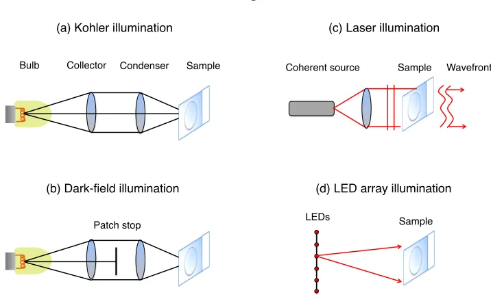
micro-scopes use Kohler illumination, as diagrammed in Fig. 1.2(a). Here, we show a trans-illumination

Kohler scheme, where light passes through the sample to the image plane. However, the same

princi-ple also extends to epi-illumination. In either case, Kohler designs use a set of lenses (a collector and

condenser lens) to spread incoherent light as evenly as possible across the sample plane. Typically,

a thermal source, such as a light bulb, creates the incoherent light. The benefits of using incoherent

illumination in a microscope are two-fold. First, a wide range of optical frequencies (i.e., colors)

reach the sample and subsequently transmit information about possible absorption, excitation, and

fluorescence at different energy levels to the detector. Second, incoherent illumination offers a slight

benefit in terms of maximum achievable image resolution, as detailed later in this thesis.

An alternative illumination geometry using an incoherent source is shown in Fig. 1.2(b). Here,

(11)

4

Sample! (a) Kohler illumination!

(b) Dark-field illumination!

(c) Laser illumination!

(d) LED array illumination!

Collector! Condenser!

Bulb!

Patch stop!

Sample! Wavefront!

Sample!

Coherent source!

[image:11.612.140.498.62.279.2]

LEDs!

Figure 1.2: Four different trans-illumination schemes that are common within microscopy. (a) Kohler illumination provides even incoherent light across the sample. (b) Dark-field illumination blocks the central rays in a Kohler setup before they reach the sample. (c) Coherent illumination is helpful, e.g., in digital holographic microscopy. (d) An LED array provides a computationally addressable, spatially coherent illumination source.

prevents all rays traveling at small angles with respect to the optical axis from reaching the sample.

As a result, only light traveling at large angles will hit the sample. This angled incident light will

not enter the objective lens unless it is diffracted by the sample. In other words, the incident light

is traveling at an angle that is too large to pass directly into the objective lens in the absence of

a sample, and must somehow interact with the sample to deflect into the lens acceptance angle.

Dark-field imaging is particularly helpful at highlighting fine sample features which diffract incident

light into a wide range of angles. We will return to this fundamental principle in Chapter 2 during

our explanation of Fourier ptychography.

Instead of using an incoherent light source, it is also possible to illuminate a sample of interest

with spatially and temporally coherent light, such as light from a laser. Spatially and temporally

coherent light can be modeled as a wave, with a defined amplitude and phase across space.

Suffi-ciently spatially coherent light helps to preserve any phase information contained within the optical

field exiting the surface of a sample (see Fig. 1.2(c)). It is possible to measure this exiting field’s

phase using digital holography or via alternative computational methods [13]. As we will detail,

knowledge of this phase is also helpful when reconstructing thick, three-dimensional samples during

tomographic measurements.

A final type of microscope illumination that will play a major role in this thesis originates from

an LED array (Figure 1.2(d)). Light from an LED lies somewhere between that originating from

(12)

nm spectral bandwidth). Furthermore, the active area of an LED is quite compact, typically on

the order of several hundred microns in diameter. Thus, it is often possible to consider light from

one distant LED as originating from a small point source that is effectively spatially coherent and

quasi-monochromatic [23] (see definition below). An array of individually addressable LEDs allows

one to turn on multiple individually coherent, yet mutually incoherent sources at a time. Or, one

may effectively shift one coherent source to different spatial locations along the illumination plane.

Note that while certainly possible, this thesis does not consider placing any optics between the LED

array and sample, or curving the LED array plane.

This variable source of LED illumination is closely related to other “structured illumination”

techniques used in microscopy. Specifically, a structured illumination setup creates and shines a

specific pattern of optical intensity onto the sample. Examples include sinusoidal stripes [17, 18]

or random speckle [19, 20]. Since structured illumination is almost always used with the goal of

fluorescent imaging in mind, the phase of the illumination light is rarely manipulated. The LED

array in Fig. 1.2(d) can be thought of as a method to provide structured illumination with a uniform

intensity across the surface of the sample, but a spatially varying phase, whose profile depends upon

the distance of the activated LED from the optical axis.

1.1.2 The sample plane

The sample plane is located directly above the illumination plane. We denote its spatial coordinates

as (x, y), which are perpendicular to the axis of propagation, z (see labels in Fig. 1.1). For the

majority of this thesis, we will consider imaging thin samples. The thin sample condition holds if

the maximum sample thicknesst obeyst <<4δ2

res/πλ, whereδres is the sampling resolution andλ is the illuminating light’s central wavelength [12]. If a sample satisfies this condition, then we may

completely summarize its interactions with light using a complex two-dimensional function,ψ(x, y).

Specifically, the amplitude of ψ(x, y) defines the amount of light absorbed by the sample at each

spatial location (x, y) when illuminated with a uniform plane wave. Likewise, the phase ofψ(x, y)

defines the spatially varying phase delay imparted by the sample to the incident plane wave. If the

sample does not strictly satisfy the above thickness condition, we often find that a 2D function still

offers a very useful sample description, up to a thickness of approximately 50µm. Chapter 8 details

how FP operates with thick samples.

1.1.3 The aperture plane

Next, the optical field exiting the surface of the sample propagates into our microscope. Here,

we adopt the common convention of treating the microscope as a generalized “black box” imaging

(13)

of microscope lenses using just an entrance pupil and an exit pupil, which are each images of the

same limiting aperture. This limiting aperture typically includes a physical stop within the system of

lenses to minimize the effect of aberrations, and to block any stray light. We define the plane of this

limiting aperture as our “aperture plane”. It may be described by an aperture function, a(x0, y0).

Here, we define (x0, y0) as the spatial coordinates at the aperture plane perpendicular to the optical

axis. Following the simple analysis in [10], it is direct to show that the coordinates (x0, y0) are the

Fourier conjugate coordinates of (x, y). In practice, when using an infinity-corrected objective lens

and tube lens to form an image, the Fourier conjugate aperture plane is located at the microscope

objective lens back focal plane.

Equivalent descriptions of microscopes sometimes rely upon the image of the aperture plane

from the point of view of the image plane (i.e., the exit pupil). We define the image of the aperture

functiona(x0, y0) from the point of view of the image plane, as the pupil function,p(x0, y0). Typically,

p(x0, y0) is equivalent to or a scaled version of the aperture function,a(x0, y0). In this thesis, we treat

the aperture and pupil functions as equivalent. Both are Fourier conjugate to the sample and image

planes. However, care should be taken in actual system analysis to ensure equality when appropriate.

1.1.4 The image plane

After passing through the microscope, our optical field of interest will terminate at the image plane.

In all imaging setups considered here, our image plane contains a digital detector array with a finite

pixel size. Each pixel will sample the intensity of the incoming optical field. This sampling process

can be described as a convolution between the incident optical field, which is band-limited, and a

pixel sampling function [16]. Through Shannon’s sampling theorem, it is thus possible to exactly

describe the intensity of the incoming optical field with the set of discrete measurements from the

detector array. A detailed analysis of the effects of pixel sampling on image formation is given in

Chapter 7 of [16].

Typical CCD and CMOS detectors contain approximately 106_-107 _{pixels, with pixel sizes that}

are in the range ofδx= 1.5−10µm. To avoid aliasing, we will always assume that the pixel sizeδx exceeds the maximum spatial frequency of incoming (coherent) light. Unless otherwise mentioned,

our experiments use a 20 megapixel Kodak KAI-29050 CCD detector with a pixel size of 5.5µm.

1.2 Relevant definitions

This thesis repeatedly characterizes the performance of microscope imaging using several related

parameters. In this section, we briefly define these common parameters for quick reference. Most of

(14)

Diagram to show FOV, NA and PSF (and magniﬁca/on?)

Image!

do! di!

l

Sample ! Aperture!

LEDs!

Field number FOV!

θi! θa!

h!

a(x') = rect(x'/w)! h(x) = sinc(xλ/NA)!

LED area a!

(a) Geometric optics parameters!

(b) Wave optics parameters!

Coherence length Lc!

CTF! PSF!

z!

x!

z!

x'!

z!

[image:14.612.197.450.238.493.2]

x!

(15)

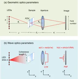
• Magnification: In an infinity-corrected microscope setup, such as those considered in this thesis, the image magnificationM is typically defined as,M =fo/ft, wherefois the objective lens focal length andft= 180 mm is the tube lens focal length. To ensure that this standard is followed by our simple microscope, and that the well-known single lens magnification definition

M =di/do also holds true, we simply setdo=fo anddi =fl= 180 mm. We maintain these equalities for the entire thesis.

• Field number and field-of-view: The field number (FN) of a microscope is defined as the diameter of the measured optical field at the intermediate image plane of a compound

microscope. In most stand-up microscopes, this corresponds to the plane of the digital detector.

We assume the optical field at the image plane extends a large distance along xand y, such

that the FN in our simple microscope is limited by the width of the digital detector. A typical

field number is FN= 26.5 mm. The field-of-view (FOV, also called field size) is the field number

de-magnified, which is its spatial extent at the image plane: FOV=FN/M.

• Numerical aperture (NA): The microscope objective numerical aperture is NA =n·sin(θa), where n is the refractive index of the medium of propagation (n = 1 in air), and θa is the maximum acceptance half-angle of the microscope objective. In our simple microscope, we

define the maximum lens acceptance half-angleθaalong the optical axis. We note that our LED array also has an effective illumination numerical aperture,N Ai, defined using the maximum possible angleθiof a plane wave generated by the most laterally displaced LED: NA =n·sin(θi)

• Impulse response and point-spread function: The impulse response of a coherent imaging system, h(x, y), defines its complex response to an idealized point source placed along the

optical axis at the sample plane. In the absence of aberrations, the shape ofh(x, y) remains

shift-invariant across the entire image plane. The function h(x, y) is given by the inverse

Fourier transform of the CTF, defined below. Typically, the CTF is a circular function in

two dimensions, and we find h(x, y) = Jinc(xλ/N A). Here, the “Jinc” function is defined as

Jinc(x) = J1(2πx)/x, where J1 is a Bessel function of the first kind, order-1. A good rule of

thumb is to assume the width of the impulse response as approximatelyλ/N A. As we detail

in Chapter 2, this width approximates the smallest resolvable sample feature when imaging

with a conventional microscope. Finally, the point-spread function of an imaging system is the

squared magnitude of the impulse response, |h(x, y)|2.

• Coherent transfer function (CTF): In a coherent imaging system, such as those con-sidered in a large part of this thesis, the CTF defines the imaging system’s response in

the spatial frequency domain. Specifically, given a sample function ψ(x, y), we may

(16)

Fourier conjugate variables of (x, y), and the hat denotes a two-dimensional Fourier

trans-form. Following principles from Fourier optics, the spatial frequency representation of the

optical field at the image plane (i.e., its Fourier transform, or spectrum), ˆg(x0, y0), is given

as, ˆg(x0, y0) = ˆψ(x0, y0)ˆh(x0, y0). Here, ˆh(x0, y0) is the imaging system CTF. A fundamental

insight from Fourier optics states that the CTF is simply a scaled version of the lens aperture

function: ˆh(x0, y0) =a(λdix0, λdiy0) [10]. Typically, we will ignore constant coordinate scaling factors when examining the behavior of our Fourier ptychographic microscope, for simplicity.

This allows us to define the coordinates of the aperture plane as simply (x0, y0), the Fourier

conjugate variables of the coordinates at the sample plane. Furthermore, we’ll also ignore any

scaling effects between the sample and image plane and will label both using (x, y), as shown

if Fig. 1.3.

• Space-bandwidth product: The space-bandwidth product of an imaging system (SP) is the total number of resolvable features it can capture. Mathematically, the SP is approximately

given by the imaging system field-of-view divided by the average width of its impulse response,

h(x, y). If the width of the impulse response varies across the image plane, as is typically the

case in most microscope objectives (due to the influence of aberrations), then this variation

must be taken into account when computing the SP. This thesis will also occasionally use a

related alternative definition of the SP of a band-limited optical system, given as the product

of the spatial extent and spatial frequency range that it can fully capture [22].

• Quasi-monochromatic: As first noted in [23], the quasi-monochromatic condition must be met if one wishes to neglect the effect of the finite spectral bandwidth of an optical field.

Specifically, if we wish to accurately assume that an optical source used within an imaging

experiment is one frequency ν, then its spectral bandwidth ∆ν must satisfy the following

inequality: ν/∆ν > nx. Here,nxis the number of pixels along one axis of the digital detector. If a source meets this condition, then one can neglect the effects of its spectral bandwidth on

the intensity values within each detected image. In our setup, a ∆ν of several nanometers is

required to fulfill the quasi-monochromatic condition, which a highly temporally coherent LED

may satisfy. Unless otherwise stated, this thesis treats each LED in our illumination array as

quasi-monochromatic.

• Coherence length: While the above quasi-monochromatic assumption offers an accurate model for the spectral response of our LED array microscope, the assumption that each LED

is an ideal point source is not accurate, in practice. Instead, we must take into account the

finite width wl of each LED, which we treat as square light source that is fully incoherent within its photon generating region. From the Van Cittert-Zernike theorem, a fully incoherent

(17)

Objective Magnification/NA/Field

number

Resolution 532 nm incident wavelength (μm)

Space-Bandwidth Product (SP)

megapixels

1.25X/0.04/26.5 8.12 21.5 MP 2X/0.08/26.5 4.06 33.5 MP 4X/0.16/26.5 2.03 33.5 MP 10X/0.3/26.5 1.08 18.9 MP 20X/0.5/26.5 0.65 13.1 MP 40X/0.75/26.5 0.43 7.4 MP

60X/0.9/26.5 0.36 4.7 MP

100X/1.3/26.5 0.25 3.5 MP

Figure 1.4: Space-bandwidth product (SP) of various microscope objectives. Although maximum resolutions vary significantly, all lenses exhibit a SP less than 50 megapixels

It is useful to define a measure of the field’s coherence [24], given by the coherence length Lc a distance z away from the LED, as Lc =λz/wl. Within this coherence length, a partially spatially coherent field remains effectively correlated with itself, and can thus be approximated

as a coherent field. In other words, a two-slit experiment will produce visible fringes up to a

slit separation of approximately Lc, after which the resulting fringes will decrease in contrast to zero.

1.3 Challenges for the standard microscope

To capture a standard microscope image, one selects any of the illumination schemes from Fig. 1.2,

illuminates the sample, forms an image of the illuminated sample on the detector, and records the

optical intensity for a finite exposure time. While commercial systems can form very sharp images

across a variety of magnifications, these snapshots still lack several key properties desired by the

experimentalist. Below, we outline several of these key properties that Fourier ptychography can

help solve, as well as some of the prior work that attempts to achieve a similar goal:

• A high space-bandwidth product (SP): As detailed in [2], the SP of an imaging system is primarily influenced by two phenomena: diffraction and aberrations. Diffraction effects are

minimized by using a larger lens (i.e., the PSF width scales inversely with the lens diameter

and numerical aperture). Unfortunately, the size of aberrations also increase linearly with size

of the lens. Thus, a tradeoff space emerges, where lenses must be highly optimized to both

achieve a sharp PSF and also provide minimal aberrations across as large a FOV as possible.

(18)

glass elements to form one microscope objective.

Due to this lens scaling law, a tradeoff space eventually emerges between image resolution

and field-of-view. Microscope objectives designed to capture very high resolution images suffer

from a narrow field-of-view, and objectives designed to image a wide field-of-view exhibit poor

resolution. Thus, all microscope systems are currently limited to a SP of approximately 50

megapixels (or less). Fig. 1.4 lists a variety of different objective lenses and the total number of

pixels (i.e., the SP) that each can capture [26]. As described in Chapter 2, Fourier ptychography

overcomes this tradeoff by first capturing a sequence of SP-limited images. Then, it fuses them

together to reconstruct an image with an effective SP of 1 gigapixel.

This lens scaling law is not limited to microscopes, but applies to all generalized imaging

systems. Several recent efforts use the principle of multi-scale lens design to overcome this

scaling law [27]. Unlike such prior work, Fourier ptychography requires variable illumination

to achieve its resolution gain, and is thus best suited to increase the SP within microscopes,

where one typically has control over the illumination source.

• Quantitative phase: Light, as an electromagnetic field, has both an amplitude and phase. All optical detectors can only directly measure the amplitude of the field (specifically, the intensity)

and not the phase. As mentioned in the introduction, optical phase can be extremely helpful.

However, these phase-sensitive techniques from the early years of microscope design (e.g.,

phase contrast and differential interference contrast) do not offer quantitative measurements,

but instead provide indirect evidence of phase variation. Quantitative phase directly measures

variations in sample thickness and index of refraction. It also enables direct removal of system

aberrations, and the ability to digitally refocus an image formed with spatially coherent light

(see below).

Measuring quantitative phase has a long history. Holography inherently relies upon recording

information connected to the phase of the sample of interest. Digital holography, like well

known in-line phase shifting technique [28], allows exact recovery of quantitative phase (up to

a constant unknown phase offset) through a sequence of four images. Computational methods,

such as phase retrieval [2, 4], offer a means to estimate the phase of a sample without requiring

a reference path and wavelength-precise shifting, but cannot always guarantee a completely

accurate solution. Finally, the transport of intensity equation (TIE) offers another useful

means to estimate phase [9, 31, 32]. However, TIE requires motion of the sample or within

the imaging system, and typically operates with transparent samples. As we show in

Chap-ters 2-4, Fourier ptychography acquires the quantitative phase of the optical field emerging

from a sample, simultaneous to improving the imaging system spatial resolution. It may also

(19)

microscope aberrations), which can be removed to form a much sharper image.

• Digital refocusing: In a standard microscope, focusing to the ideal plane of interest can be a challenge. Often, the sample is not perfectly flat at different areas across the sample plane,

causing the image to come into focus at different depths along the optical axis, z. Frequent

users of microscopes, such as pathologists, are well aware of the challenges surrounding manual

focusing. One computational imaging technique, termed light field microscopy, replaces manual

refocusing with limited digital image refocusability, post-capture [5, 34]. However, light field

images offer a significantly limited resolution, and require the insertion of a microlens array

near the image plane, thus necessitating a customized microscope body.

Once one acquires both the amplitude and phase of the optical field at the detector, it is simple

to digitally refocus the field through a wide range of axial planes, by computational propagation

(e.g., using the angular spectrum method [10]). Computational propagation enables direct

refocusing of FP images while maintaining their sub-micron resolution. In addition, it is

common for a sample to occupy an unknown defocus plane, or perhaps lie at an unknown tilt.

During FP reconstruction, we can additionally solve for these unknown placements and tilts to

offer a sharp image across a significantly extended depth-of-field (up to 75 times a comparable

objective lens, as discussed in Chapter 3).

• Aberration removal: As noted above, all lenses exhibit aberrations, which deteriorate im-age quality. Over the past half-century, many unique aberration characterization methods

have been reported [36–38]. These methods typically attempt to estimate the phase

devia-tions or the frequency response of the optical system under testing. Several relatively simple

noninterferometric procedures utilize a Shack-Hartmann wavefront sensor [38], consisting of

an array of microlenses that each focus light onto a detector. Despite offering high accuracy,

measuring aberrations with a Shack-Hartmann sensor often requires considerable modification

to an existing optical setup. Alternatively, wavefront aberrations can be inferred directly from

intensity measurements, by relying upon phase retrieval procedures [24]. Such computational

methods typically require capturing multiple images, while inducing some unknown change to

the optical system between each capture (i.e., while applying “measurement diversity” [24,40]).

As we will show in this thesis, Fourier ptychography provides a very useful form

measure-ment diversity through its variable illumination source. This enables robust computational

estimation of system aberrations and their subsequent removal, which significantly improves

the effective resolution of our final image reconstructions.

(20)

representation of a thick sample. This inversion process closely resembles diffraction

tomog-raphy (DT) [14]. Unlike in all prior DT setups, FP does not measure the phase of the optical

field. This allows one to use a standard microscope, outfitted with an LED array and computer,

to computationally recover a quantitative measurement of the complex index of refraction of

a thick sample of interest (t > 100µm), from throughout its volume, at a micrometer-scale

resolution.

There is one key item that many current microscope experiments currently focus on that is

missing from the above list: improving fluorescent image capture. For example, recent fluorescent

particle localization techniques, such as PALM and STORM, can exceed standard microscope

resolu-tion limits [42]. Likewise, structured illuminaresolu-tion methods may yield similarly unbounded resoluresolu-tion

gains [18]. Standard Fourier ptychography assumes all optical interactions are coherent (i.e., a phase

relationship is preserved, at least locally). Fluorescent excitation does not preserve phase and thus

will not obey the interactions FP predicts. While it is possible to adapt the principle of Fourier

ptychography to achieve fluorescent resolution enhancement [43], this thesis will not discuss in

de-tail this possible direction. We hope the reader keeps this important point in mind throughout the

following discussions.

Here is an outline for the rest of this thesis. In Chapter 2, we will overview the principle of

FP in an optical microscope, from a Fourier optics perspective. In Chapter 3, we will discuss the

process of Fourier ptychographic image reconstruction using a phase retrieval algorithm. In Chapter

4, we will examine the quantitative accuracy of Fourier ptychographic phase reconstruction. We also

briefly visit several applications of measuring high-resolution phase, including the ability to digitally

refocus images, remove aberrations, and determine structural information regarding biological tissue.

In Chapter 5, we will connect Fourier ptychography to its “standard” counterpart in X-ray imaging,

ptychography, using a unique mathematical phase-space model. This model highlights the role of

partial coherence during data acquisition and image reconstruction. In Chapter 6, we will present a

convex approach to process both standard and Fourier ptychographic data, which performs better

in the presence of noise than prior reconstruction techniques. In Chapter 7, we implement Fourier

ptychography within a conventional camera setup, which helps remove unknown aberrations from

a final reconstructed image. Finally, in Chapter 8, we apply the principle of ptychography to

reconstruct thick samples, using a process that resembles diffraction tomography but does not require

(21)

Bibliography

[1] R. M. Allen,The Microscope(Chapman and Hall Limited, 1940).

[2] F. Zernike, “Beugungstheorie des Schneidenverfahrens und seiner verbesserten Form, der

Phasenkontrastmethode,” Physica 1, 689–704 (1934)

[3] F. Zernike, “How I Discovered Phase Contrast”. Science 121, 345–349 (1955).

[4] F. Zernike, “Phase contrast, a new method for the microscopic observation of transparent

objects part I”, Physica 9 (7), 686–698 (1942).

[5] G. Nomarski, “Interferential polarizing device for study of phase objects,” US Patent

US-2924142A (1960).

[6] M. Minsky, “Microscopy apparatus,” US Patent US-3013467A (1961).

[7] Z. Huang, “A Review of Progress in Clinical Photodynamic Therapy,” Technology in Cancer

Research and Treatment, 4(3), 283–293 (2005).

[8] G. C. R. Ellis-Davies, “Caged compounds: photorelease technology for control of cellular

chem-istry and physiology,” Nat. Meth. 4(8), 619–628 (2007).

[9] F. Zhang et al., “Optogenetic interrogation of neural circuits: technology for probing

mam-malian brain structures,” Nat. Protocols 5(3), 439–456 (2010).

[10] J. W. Lichtman and J. A. Conchello, “Fluorescence microscopy,” Nat. Meth. 2(12), 910–919

(2005).

[11] S. W. Hell and J. Wichmann, “Breaking the diffraction resolution limit by stimulated emission:

Stimulated-emission-depletion fluorescence microscopy,” Opt. Lett. 19(11), 780-782 (1994).

[12] G. Zheng, R. Horstmeyer and C. Yang, “Wide-field, high-resolution Fourier ptychographic

microscopy,” Nature Photon.7, 739–745 (2013).

(22)

[14] K. Nugent, “Coherent methods in the X-ray sciences,” Adv. Phys.59(1), 1–99 (2010).

[15] J. Goodman,Introduction to Fourier Optics(McGraw-Hill, 1996). [16] D. Brady,Optical Imaging and Spectroscopy (John Wiley & Sons, 2009).

[17] M. Gustafsson, “Surpassing the lateral resolution limit by a factor of two using structured

illumination microscopy,” J. Microsc. 198, 82–87 (2000).

[18] M. G. L. Gustafsson, “Nonlinear structured-illumination microscopy: wide-field fluorescence

imaging with theoretically unlimited resolution,” Proc. Nat. Acad. Sci. 102, 13081–13086 (2005).

[19] J. Garcia, Z. Zalevsky and D. Fixler, “Synthetic aperture superresolution by speckle pattern

projection,” Opt. Express 13, 6073–6078 (2005).

[20] E. Mundry et al., “Structured illumination microscopy using unknown speckle patterns,” Nat.

Photonics 6, 312–315 (2012).

[21] P. D. Nellist, B. C. McCallum and J. M. Rodenburg, “Resolution beyond the ‘infromation limit’

in transmission electron microscopy,” Nature374, 630–632 (1995).

[22] A. W. Lohmann, R.G. Dorsch, D. Mendlovic, Z Zalevsky, and C. Ferreira, “Spacebandwidth

product of optical signals and systems,” J. Opt. Soc. Am. A 13, 470473 (1996).

[23] A. W. Lohmann, “Matched Filtering with Self-Luminous Objects, Appl. Opt. 7, 561563 (1968).

[24] J. Goodman,Statistical Optics(John Wiley and Sons, 2000).

[25] A. W. Lohmann, “Scaling laws for lens systems,” Appl. Opt. 28, 4996-4998 (1989)

[26] G. Zheng, X. Ou, R. Horstmeyer, J. Chung and C. Yang, “Fourier ptychographic microscopy:

creating a gigapixel microscope for biomedicine,” Optics and Photonics News 25(4), 26–33

(2014).

[27] D. Brady et al., “Multiscale gigapixel photography”. Nature 486, 386389 (2012).

[28] R. Gerchberg, “A practical algorithm for the determination of phase from image and diffraction

plane pictures,” Optik (Stuttg.) 35, 237 (1972).

[29] J. R. Fienup, “Phase retrieval algorithms: a comparison,” Appl. Opt. 21(15), 2758–2769 (1982).

[30] I. Yamaguchi and T. Zhang, “Phase-shifting digital holography,” Opt. Lett.22(16) 1268–1270

(1997).

[31] N. Streibl, “Phase imaging by the transport equation of intensity,” Opt. Commun. 49(1), 6–10

(23)

[32] T. E. Gureyev and K. A. Nugent, “Rapid quantitative phase imaging using the transport of

intensity equation,” Opt. Commun. 133, 339–346 (1997).

[33] L. Waller, L. Tian, and G. Barbastathis, “Transport of Intensity phase-amplitude imaging with

higher order intensity derivatives,” Opt. Express 18(12), 12552–12561 (2010).

[34] M. Levoy, R. Ng, A. Adams, M. Footer and M. Horowitz, “Light field microscopy,” ACM Trans.

Graphics 25, 924–934 (2006).

[35] M. Levoy, Z. Zhang and I. McDowall, “Recording and controlling the 4D light field in a

micro-scope using microlens arrays,”. J. Microsc. 235, 144–162 (2009).

[36] M. Takeda and S. Kobayashi, “Lateral aberration measurements with a digital Talbot

interfer-ometer,” Appl. Opt. 23(11), 1760–1764 (1984).

[37] S. Gong and S. S. Hsu, “Aberration measurement using axial intensity,” Opt. Eng. 33(4), 1176–

1186 (1994).

[38] J. L. Beverage, R. V. Shack, and M. R. Descour, “Measurement of the three-dimensional

mi-croscope point spread function using a Shack-Hartmann wavefront sensor,” J. Microsc. 205(1),

61–75 (2002).

[39] R. G. Paxman, T. J. Schulz, and J. R. Fienup, “Joint estimation of object and aberrations by

using phase diversity,” JOSA A 9(7), 10721085 (1992).

[40] M. Guizar-Sicairos and J. R. Fienup, “Phase retrieval with transverse translation diversity: a

nonlinear optimization approach,” Opt. Express 16, 7264–7278 (2008).

[41] V. Lauer, “New approach to optical diffraction tomography yielding a vector equation of

diffrac-tion tomography and a novel tomographic microscope,” Journal of Microscopy 205, 165–176

(2002).

[42] M.A. Thompson, M.D. Lew, and W.E. Moerner, “Extending microscopic resolution with

single-molecule imaging and active control,” Annu Rev Biophys 41, 321–42 (2012).

[43] S. Dong, P. Nanda, K. Guo, and G. Zheng, “High-resolution fluorescence imaging via

(24)

Chapter 2

Fourier ptychography for gigapixel

imaging

In this chapter, we use our model of a simple microscope from Chapter 1 to explain the principle of

Fourier ptychography (FP). The goal of FP is to computationally resolve an image containing one

billion pixels (i.e., a gigapixel) from a sequence of low-resolution measurements. To begin, we will

first motivate the concept of improving resolution by means of a shifting illumination source. Then

we will present a mathematical model to explain the process of Fourier ptychographic data capture.

We will limit our discussion here to a two-dimensional optical geometry (i.e., one spatial axis that is

orthogonal to the axis of optical propagation). At the end of this chapter, we will discuss extension

to a three-dimensional setup.

2.1 Resolution improvement through shifting illumination

As noted in Chapter 1, a microscope’s numerical aperture (NA) defines its resolution performance.

Specifically, the minimum resolvable feature within a standard microscope is approximated as

λ/NA = λ/sinθ. Here, we assume the standard microscope is under coherent illumination (from

a distant point source) and operates within air, which sets the index of refraction term within the

NA equal to 1. As diagrammed in Fig.2.1(a), the half-angleθ denotes the largest cone of

wavevec-tors (i.e., rays) that can pass from the sample and into the imaging lens, and defines the system’s

maximum resolvable feature.

Most biological samples of interest contain many micrometer-scale features that diffract light

into a large cone of wavevectors. In Fig.2.1(a), this larger green cone subtends an angleω > θ and

is thus not completely captured by the microscope. To resolve smaller features at the image plane,

we would ideally like to capture all of the rays within this large green cone. Specifically, we would

like to somehow keep the low-NA objective lens in Fig.2.1 for imaging, since it offers a very large

(25)

Detector! Microscope

lens (red)!

Sample! Illumination

source!

θ"

(a) Direct illumination! (b) Angled illumination!

φ_"

θ"

Illuminate n

LEDs! Capture n images!

Shift

illumination! Tilted ray cone!

(c) LED illumination for multiple angles!

shift!

ω

_ω

φ

_"

Figure 2.1: Capturing a wider cone of wavevectors. (a) A standard microscope with a limited NA = nsinθ captures only the red cone of rays emerging at half-angle θ from the sample. An ideal microscope can capture the wide green cone of rays emerging at angle ω. (b) By shifting the illumination source, we can rotate the green cone of rays emerging from the thin sample surface. Now, a different segment of the green cone will pass through the fixed “red” aperture. (c) FP uses an array of nLEDs to shift the wide green cone of rays ntimes. Each time the cone is shifted, a unique image is captured. From the set ofnimages, the computational goal of FP is to synthesize an image with a larger NA, as if it originated from a lens that could originally capture the wide green cone of rays.

high resolution. The combination of both a wide image FOV and high resolution will lead to a large

space-bandwidth product (SP) system.

To capture the large green cone of rays through our low-NA microscope objective lens, Fourier

ptychography shifts its illumination source, as diagrammed in Fig.2.1(b). A shifting illumination

source will illuminate the sample from a variable angle, φ. If the sample is thin, this will cause

the green cone of rays emerging from the sample surface to also rotate, by the same angle φ. At

the microscope lens, the green cone of rays will subsequently shift laterally by a finite distance. As

is clear in Fig.2.1(b), the shifted source will cause a different segment of the green cone to pass

through our fixed microscope objective lens (denoted by the red circle). As we shift the illumination

source across many different positions, then the entire green cone of rays, albeit at different points

in time, will pass through the fixed objective lens and subsequently propagate to the detector. If we

capture an image of the optical field that passes through the objective lens at each unique location

of the shifted optical source, then we have conceptually captured information corresponding to the

entire green cone of rays. The goal of Fourier ptychography is to use this set of captured images

to computationally recover a single image that appears to have passed through a “synthetic” lens,

whose effective size extends across the entire green cone of rays (i.e., a new lens with an acceptance

half-angleω). This synthesized image will now have a much higher resolution – its smallest resolvable

element will now approachλ/sinω.

Instead of actually shifting an illumination source laterally, Fourier ptychography typically uses

(26)

Image g(x)!

l

Sample ψ(x)! Aperture a(x')!

LEDs!

θj" θa"

r"

jth source!

S(x)! A(x')!

L(x')! D(x)!

r"

jth source!

(a) FP setup!

(b) FP, wave optics!

Plane wave!

Shifted spectrum!

exp(ikxpj)!!ψ(x)!

Sample! Image!

F [a(x)ψ(x-pj)]! 2! ψ(x-pj)!

[image:26.612.180.471.79.387.2]

p_j

Figure 2.2: Optical diagram for our simple 2D FP setup, with (a) planes and distances of interest labeled, and (b) wave optics descriptions of the resulting optical field at each plane of interest. The final image is both a function of space (x) and incident illumination angle (pj). Each captured image thus forms one column of our FP data matrix,g(x, pj).

solidify the above concept of Fourier ptychographic data capture, before explaining how we transform

the data into a high resolution image, in Chapter 3.

2.2 Mathematical model of Fourier ptychography

We mathematically model our microscope imaging system in two dimensions (x, z), for simplicity. We

assume that a distant planeL(x0) containsqdifferent quasi-monochromatic optical sources (central

wavelengthλ) evenly distributed alongx0 with a spacingr. We assume each optical source acts as

an effective point emitter that illuminates a sample ψ(x) at a plane S(x) a large distance l away

fromL(x0). Under this assumption, thejth source illuminates the sample with a spatially coherent

(27)

field exiting the thin sample as the sample-plane wave product,

s(x, pj) =ψ(x)eikxpj_, _(2.1)

where the wavenumber k = 2π/λ and pj = sinθj describes the off-axis angle of the jth optical source.

The jth illuminated sample field s(x, pj) then enters an imaging system with a low numerical aperture (NA). Neglecting scaling factors and a quadratic phase factor for simplicity, Fourier optics

gives the field at the imaging system aperture plane,A(x0), as

F[s(x, pj)] = ˆψ(x0−pj). (2.2)

Here,F represents the Fourier transform between conjugate variablesxandx0, and ˆψis the Fourier transform ofψ. Eq. 2.2 uses the Fourier shift property to show that the spectrum of a thin sample,

when illuminated by a plane wave at an angle given by the inverse sine ofpj, will shift bypjlaterally across the imaging system’s aperture plane.

The shifted spectrum field ˆψ(x0−pj) is then modulated by the aperture function of the imaging system,a(x0), which acts as a low-pass filter. As outlined in Chapter 1, the aperture functiona(x0) is

typically a physical stop placed at the back focal plane of the microscope objective. It usually exhibits

a circular shape in two dimensions. In the conceptual schematic of FP in Fig. 2.2,a(x0_{) is the limited}

width of the transparent lens area at the aperture plane, which may be mathematically expressed as

a rect function. The shape ofa(x0) is directly proportional to the imaging system coherent transfer

function (CTF), which in turn defines the lens cutoff spatial frequency, its maximum acceptance

angle, and thus also its NA.

It is now useful to consider the sample spectrum ˆψ discretized into n pixels with a maximum

spatial frequency k. Following the Nyquist-Shannon sampling theorem, since our optical signal is

now bandlimited to the aperture area a(x0), this discretization process is exact. We denote the

bandpass cutoff of the aperture function a as k·m/n, where m is an integer less than n. The modulation of ˆψbyaresults in a field characterized bymdiscrete samples, which propagates to the

camera imaging plane,D(x). Here, the digital detector critically samples the incident field using an

m-pixel digital detector (e.g., a CCD or CMOS detector, which we assume has a perfect fill factor).

This forms a reduced-resolution intensity image,g(x, pj):

g(x, pj) =

F

h

a(x0) ˆψ(x0−pj)i 2

. (2.3)

Here, we use the subscriptjto denote that this image is formed by thejth LED. By turning on one

(28)

LED Array

Sample ψ(x,y)

Aperture a(x',y')

Image g(x,y,pjx,pjy)

L(x',y')

S(x,y)

A(x',y')

Detector D(x,y)

θ_j

Shift jxr

Low-resolution image set g

High-resolution complex sample ψ

Fourier Ptychography

… …

intensity intensity

phase

0! 2π!

Fourier Ptychography Setup

[image:28.612.176.469.82.381.2]

Shift jyr

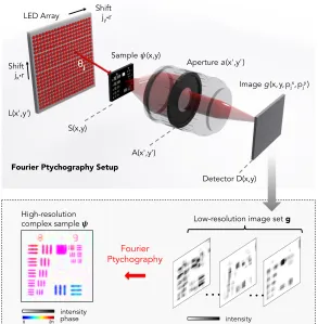
Figure 2.3: Optical diagram for an example FP setup in three dimensions, including all of the same parameters and planes as shown in Fig. 2.2. (bottom) Actual raw data and resulting reconstruction of a resolution target, demonstrating a 25X increase in microscope resolution and the simultaneous acquisition of the optical phase from the sample plane.

ptychography data matrix, g(x, pj). Thejth column of this data matrix contains a low-resolution image of the sample intensity while it is under illumination from thejth optical source.

The goal of Fourier ptychographic post-processing is to reconstruct a high-resolution (n-pixel)

complex spectrum, ˆψ(x0), from the multiple low-resolution (m-pixel) intensity measurements

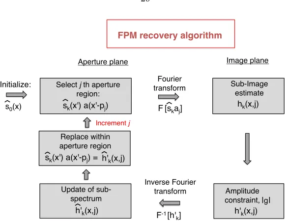
con-tained within the data matrixg(x, pj). Once ˆψis found, an inverse-Fourier transform will yield the desired complex sample reconstruction, ψ. As we will explain in the next chapter, most current

ptychography setups solve this inverse problem using an alternating projections (AP) algorithm:

af-ter initializing a complex sample estimate,ψ0, iterative constraints help forceψ0to obey all known

physical conditions. First, its amplitude is forced to obey the set of measured intensities from the

de-tector plane (i.e., the values ing). Second, its spectrum ˆψ0is forced to lie within a known support in

the plane that is Fourier conjugate to the detector. Different projection operators and update rules

are available, but are closely related [4, 5, 46]. It is also possible to solve the inverse ptychography

problem with a convex program, which this thesis examines in detail in Chapter 6.

(29)

Image 1!

Image 2!

Image 3!

g'(x',1-3)!

Detect 3 complex images:!

Inverse Fourier transform! Synthesized spectrum

es2mate, ψ0(x')

[image:29.612.178.473.67.296.2]

LEDs! Sample! Aperture!

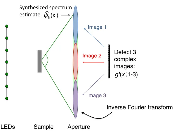
Figure 2.4: Conceptual outline of using a synthetic aperture to improve image resolution. If each detected image in the sequence of low-resolution measurements also captures the phase of the optical field, then reconstruction is direct. Each detected image is inverse Fourier transformed to the aperture plane (to form the values of the optical field within each colored circle). These three Fourier transforms are then stitched together, side-by-side (to form the large green circle). An inverse Fourier transform of this synthesized spectrum yields the desired high-resolution complex image. Unfortunately, the phase of light is not detected by standard optical pixel arrays, which requires us to use a slightly more involved high-resolution image reconstruction procedure, as outlined in the next chapter.

matrix in Eq. 6.2, we note that the above discussion easily generalizes to a three-dimensional

geome-try. This extension is diagrammed in Fig. 2.3, where all functions ofxandx0 are now also functions

of y and y0, respectively. LED scanning is performed along two dimensions separately. Combined

with two-dimensional images, this creates a four-dimensional data matrix,g(x, y, px j, p

y

j), where now

r/2≤jy ≤r/2 is the counter for LEDs along the second axis, where a total of q×r LEDs are in the possibly rectangular array.

2.3 Reconstruction goals and extensions

The goal of ptychographic recovery is to convert the acquired data matrix into a complex sample

reconstruction with improved resolution. It will be useful at several points throughout this thesis

to return to the above data matrix picture, as several different algorithms are discussed. Here, we

briefly outline one related strategy to help connect the above concepts to our final goal of resolution

improvement.

First, let us assume for simplicity that our digital detector can also detect the phase of incident

(30)

if the phase were detected, then our data matrix would no longer be squared:

g0(x, pj) =Fha(x0) ˆψ(x0−pj)i. (2.4)

Furthermore, let us assume that each captured image originated from a unique but adjacent (i.e.,

non-overlapping) region of the spectrum, ˆψ(x0). In other words, we assume that our LEDs are arranged

such that the angular shift they impart to the spectrum at each step,pj−pj−1, is equal to the total extent of the aperture in the Fourier domain,k·m/n. This ideal condition is diagrammed in Fig. 2.4. Under these two assumptions, the recovery of a high resolution image from our measurements in the

data matrix would require three straightforward steps:

• Inverse Fourier transform each image in the complex data matrix in Eq. 2.4 to recover each associated spectrum “tile”, ˆg0(x, pj) =a(x0) ˆψ(x0−pj).

• Form one long spectrum estimate vector, ˆψ0(x0), by arranging each spectrum tile from the data matrix adjacent to one another. For all j, take the spectrum tile a(x0) ˆψ(x0−pj), and place it in ˆψ0 starting at entry (j−1)·k·m/n, and ending at entryj·k·m/n. This spectrum synthesis process is diagrammed in Fig. 2.4.

• After all spectrum tiles have been concatenated together to form ˆψ0(x0), take the inverse Fourier transform of ˆψ0(x0) to recover the high resolution complex sample estimate,ψ0(x).

This simple inversion process, in the absence of noise, allows for exact recovery of a high resolution

image from a sequence of low-resolution complex image measurements. The entire process of low

resolution capture and high resolution synthesis is commonly referred to as “synthetic aperture”

imaging. Many examples of synthetic aperture imaging arise in the area of remote sensing, which

often operates within the microwave and radio regimes, where the phase of the incident field is easily

measured on a digital detector. It is also possible to implement the same concept in optical setups,

using holographic techniques to determine the phase of each individual low-resolution image [4, 5, 7,

8, 8–16].

Since it is not possible to directly measure phase within a standard microscope, synthetic aperture

imaging will not help us directly achieve our goal of gigapixel image formation. In the next chapter,

we detail how Fourier ptychography applies a phase retrieval algorithm to overcome this barrier and

(31)

Bibliography

[1] J. R. Fienup, “Phase retrieval algorithms: a comparison,” Appl. Opt. 21(15), 2758–2769 (1982).

[2] S. Marchesini, “A unified evaluation of iterative projection algorithms for phase retrieval,” Rev.

Sci. Instrum.78, 011301 (2007)

[3] P. Godard, M. Allain, V. Chamard and J. Rodenburg, “Noise models for low counting rate

coherent diffraction imaging,” Opt. Express 20 25914–25934 (2014).

[4] T. Turpin, L. Gesell, J. Lapides and C. Price, “Theory of the synthetic aperture microscope”.

Proc. SPIE 2566, 230–240 (1995).

[5] J. Di et al., “High resolution digital holographic microscopy with a wide field of view based

on a synthetic aperture technique and use of linear CCD scanning,” Appl. Opt. 47, 5654–5659

(2008).

[6] T. R. Hillman, T. Gutzler, S. A. Alexandrov and D. D. Sampson, “High-resolution, wide-field

object reconstruction with synthetic aperture Fourier holographic optical microscopy”. Opt.

Express 17, 7873–7892 (2009).

[7] L. Granero, V. Mico, Z. Zalevsky and J Garcia, “Synthetic aperture superresolved microscopy in

digital lensless Fourier holography by time and angular multiplexing of the object information,”

Appl. Opt. 49, 845–857 (2010).

[8] M. Kim et al., “High-speed synthetic aperture microscopy for live cell imaging,” Opt. Lett. 36,

148–150 (2011).

[9] C. J. Schwarz, Y. Kuznetsova and S. Brueck, “Imaging interferometric microscopy,” Opt. Lett.

28, 1424–1426 (2003).

[10] P. Feng, X. Wen and R. Lu, “Long-working-distance synthetic aperture Fresnel off-axis digital

holography,” Opt. Express 17, 5473–5480 (2009).

[11] V. Mico, Z. Zalevsky, P. Garcia-Martinez and J. Garcia, “Synthetic aperture superresolution

(32)

[12] C. Yuan, H. Zhai, and H. Liu, “Angular multiplexing in pulsed digital holography for aperture

synthesis,” Opt. Lett. 33, 2356–2358 (2008).

[13] V. Mico, Z. Zalevsky, and J. Garcia, “Synthetic aperture microscopy using off-axis illumination

and polarization coding,” Opt. Commun. 276, 209–217 (2007).

[14] A. E. Tippie, A. Kumar and J. R. Fienup, “High-resolution synthetic-aperture digital

hologra-phy with digital phase and pupil correction,” Opt. Express 19, 12027–12038 (2011).

[15] T. Gutzler, T. R. Hillman, S. A. Alexandrov and D. D. Sampson, “Coherent aperture-synthesis,

wide-field, high-resolution holographic microscopy of biological tissue,” Opt. Lett. 35, 1136–1138

(2010).

[16] S. A. Alexandrov, T. R. Hillman, T. Gutzler and D. D. Sampson, “Synthetic aperture Fourier

(33)

Chapter 3

Fourier ptychographic image

reconstruction

In Chapter 2, we derived an expression for the data matrix in Fourier ptychography (see Eq. 6.2).

We also saw that if the phase of the data matrix elements is known, then a synthetic aperture

tech-nique can recover a high-resolution microscope image from its set of low-resolution measurements.

Since the phase of each low-resolution measurement is not known, the inverse problem of resolution

enhancement becomes more challenging. In this chapter, we detail how to use an iterative phase

retrieval algorithm to accurately solve this inverse problem.

3.1 The phase retrieval algorithm

The problem of recovering a discretized complex signal (i.e., its amplitudes and phases) from

knowl-edge of just its amplitudes has a long history. Within the context of optics, one of the first successful

attempts to solve this problem was initiated by Gerchburg and Saxton in the 1970’s [2]. In this

sec-tion, we outline their general computational strategy, described within the context of our microscope.

We refer to this general class of algorithm as a “phase retrieval” method.

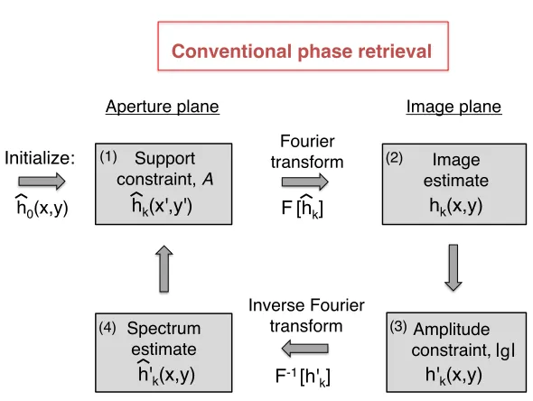
Here, we explain the simple “error reduction” (ER) phase retrieval algorithm [4], although one

of many related strategies may also be used [46]. Phase retrieval often iteratively projects an initial

estimate of the unknown complex sample, which we will define as hk(x, y) = h0(x, y), onto two constraints in two different domains. Here, the subscript k indicates the estimate is in the kth

iteration of our iterative solution process. One constraint is always the measured signal amplitudes,

which in the case of our microscope is at the image plane (i.e., the square root of the measured

intensities in the spatial domain). To begin, let us consider just one image from our microscope,

|g(x, y)|, which results from illuminating the sample from directly below with the centered LED. To determine the sample’s unknown phase values, it is common in coherent imaging to use as

(34)

Support constraint, A_!

h_k(x',y')!

h₀(x,y)!

Initialize:!

Aperture plane! Image plane!

F[h_k]!

Fourier transform!

F-1_[h' k]!

Image estimate!

h_k(x,y)!

(2) (1)

h'_k(x,y)!

(3) Spectrum

estimate! h'_k(x,y)!

(4)

| |!

Conventional phase retrieval!

Amplitude constraint, !g! Inverse Fourier

[image:34.612.174.469.77.299.2]

transform!

Figure 3.1: The ER phase retrieval algorithm for coherent imaging. Each step is detailed in the text.

constitutes additional a-priori signal knowledge, and is needed for our algorithm to accurately solve

the inverse phase retrieval problem. When imaging, one often knows the shape and extent of

the imaging system aperture function, a(x0, y0), which is almost always zero past a certain cutoff

frequency. Thus, one has a-priori knowledge that the Fourier transform of the unknown signal

estimate, ˆhk(x0, y0) must be zero outside a certain region, or in other words must be a band-limited signal. Occasionally (but not always), knowledge of the signal amplitudes and the extent of its

band-limited support is sufficient to accurately recover the unknown optical phase at the image

plane.

ER phase retrieval uses both the first “amplitude” and the second “support” constraint to

iter-atively encourage an initial signal estimate to converge to a solution containing the correct phase

values (see diagram in Fig. 3.1). First, ER initializes an estimate of the complex sample spectrum,

ˆ

h0(x0, y0), at the aperture plane. Second, ER digitally propagates this estimate to the image plane.

Following the description of our microscope from Chapter 2, propagation to the image plane is given

by a Fourier transform: hk(x, y) =F[ˆhk(x0, y0)]. Again, khere denotes the kth iterative loop, for 0≤k≤niterations, and we continue to use the “hat” to denote the signal spectrum at the aperture plane. Next, ER enforces the amplitude constraint at the image plane. It replaces the amplitudes

ofhk(x, y) with the experimentally measured amplitudes at the detector,|g(x, y)|:

h0k(x, y) =|g(x, y)|

hk(x, y)

|hk(x, y)|. (3.1)