Options valuation

Munich Personal RePEc Archive

Options valuation.

ilya, gikhman

2005

Options valuation.

Gikhman Ilya

6077 Ivy Woods Court Mason, OH 45040 ph: (513) 573 - 9348

e-mail: [email protected]

Abstract. This paper deals with the option-pricing problem. In the first part of the paper we study in details the discrete setting of the option-pricing problem usually referred to as the binomial scheme. We highlight basic differences between the old and the new approaches. The main qualitative distinction of the new pricing approach from either binomial or Black Scholes’s is that it represents the option price as a stochastic process. This stochastic interpretation can not give straightforward advantage for an investor due to stochastic setting of the pricing problem. The new approach explicitly states that the options price is more risky than represented by binomial scheme or Black Scholes theory. To highlight the difference between stochastic and deterministic option price definitions note that if a deterministic value is interpreted as a perfect or fair price we can comment that the stochastic interpretation provides this number or any other with the probability that real world option value at maturity will be bellow chosen number. This probability is a pricing risk of the option. Thus with an investor’s motivation of the option pricing the stochastic approach gives information about the risk taking. The investor analyzing option price and corresponding risk makes a decision to purchase the option or not.

Continuous setting will be considered in the second part of the paper following [1]. A significant conclusion can be drawn from the new approach. It is shown that either binomial or Black-Scholes solutions of the option pricing problem have serious drawbacks. In particular, the binomial scheme establishes the unique price for a stock that takes two values and strike price K, Sd < K < Su. According the binomial scheme this

‘fair’ price does not depends on real probabilities. Thus two options with that promise fixed income at maturity with probability close to 1 or 0 do have the same price. This of course does not have any sense. From this follows that there is no sense in using either neutral probabilities or ‘neutral world’ in options applications for valuation interest rates or credit derivatives either theoretically or numerically.

Key words: alternative option pricing, exotics, binomial scheme, continuous time, Black Scholes equation, stochastic price.

Discrete time option valuation.

To achieve proper perspectives in studying the option pricing let us begin by reviewing a discrete form and then we comment the risk-neutral probability construction. In two

periods economy let us denote the current date by 0 and the maturity date by 1. The

payoff to the European call option is defined as

$ max ( S ( 1 ) – K , 0 )

where constant K is a strike price. To begin with option pricing, we first specify the meaning of an “option price ”.

When underlying security is supposed to be stochastic two questions may arise concerning the binomial scheme. It should be clear that the method of an option price should not depend on either values of the underline security nor the distribution of underlying security. What do depend on these parameters are the option values which have to be calculated.

Let us specify an option pricing framework. Suppose a security can only move up or down; the price is then designated as Su and Sd respectively. If the security price goes

up the call option has a value Cu; if it goes down, the call option has a value Cd . The

value of the call option if the security rises is Cu = max { Su – K , 0 }, and if the security

falls, the value is Cd = max { Sd – K , 0 }. Suppose the investor is going to construct a

hedge position such as the payoff B stays the same no matter which way the security

moves. The initial position would be to hold the security, plus h units of the call option:

Bo = So + h C

The hedge ratio, h is chosen so that the ending payoff, or value B is the same no matter which way the security price moves. We establish the relationship that allows to find a unique value of h that will give a fixed payoff. Thus, the ending payoff is

B = Su + h Cu = Sd + h Cd (1.1)

The hedge position creates a less risky payoff. Solving the equation for h , the value:

h = - [ Su - Sd ] [Cu - Cd ] - 1 (1.2)

One other important thing should be noted about the hedge position. Because the ending payoff is fixed, or certain, it must be related to the annualized riskless rate r and maturity

T. This is the present value of the ending payoff. B should be equal to the investment made to construct it:

Thus,

C = ( 1 + r t ) – 1 [ πCu + ( 1 – π) Cd] (1.3)

where 0 ≤π ≤ 1 and

π = [ So( 1 + r t ) - Sd ] [ Su - Sd ] – 1 (1.4)

If the option is worth less than this amount, the investor could make a greater return than on the risk free rate. In the case where the interest rate is continuously compounded the value ( 1 + r t ) should be replaced by exp r t. The expression (1.3) is what is referred to as risk-neutral pricing and probabilities π and ( 1 – π) are often referred to as risk-neutral probabilities or equivalent martingale probabilities. We examine the option pricing formula (1.3) from the two points of view. Let’s recall option pricing problem solution. We introduce a construction of the European call option problem using the Black-Scholes approach.

Let w ( t ) be one-dimensional Wiener process and stock price S ( t ) is the solution to the equation

d S ( t ) = µ S ( t ) d t + σ S ( t ) d w( t ) (1.5)

The European Call option on security S ( t ) over a given interval [ t , T ] is an

agreement of buying shares at $ max ( S ( T; t, x ) – K , 0 ) at maturity T , which is also

known as the expiration date. Constant K is a pre-established strike price. The European

Put option gives the buyer the right to sell shares at $ max ( S ( T; t, x ) – K , 0 ). Here

S ( T; t , x ) is the solution of (1.1 ), such that S ( t; t, x ) = x.The act of making this transaction is referred to as exercising an option. Black and Scholes gave the definition of the European call option price. By definition it is a nonrandom function that is equal to the value of the portfolio containing a certain number of stocks and bonds. In B&S interpretation, a bond is a financial instrument that is governed by equation

d B ( t ) = r B ( t ) d t (1.6)

where r is a known constant interest rate.

In the simple deterministic example below we show that popular derivatives pricing models, including Black Scholes' lead to arbitrage opportunity and therefore can not be used. Then we show that the mathematical derivation of the Black Scholes equation is also incorrect. The solution of the Black Scholes equation (BSE)

∂t C ( t , x ) + r x ∂x C ( t , x ) + ½ σ ² x ² ∂x x C ( t , x ) = 0 (1.7)

C ( T , x ) = max ( x – K , 0 )

represents the value of the European call option contract on a common stock, which price is governed by the equation (1.5). Using probabilistic representation of the solution for the parabolic Cauchy problem, the Black Scholes equation solution can be written in the form

C ( t , x ) = E exp – r ( T – t ) max ( η ( T ; t , x ) – K , 0 ) (1.8)

where η ( l ; t , x ), l > t is the solution of the Ito equation

d η ( l ) = r η ( l ) d l + σ η ( l ) d w ( l )

such that η ( t ) = x.

It seems instructive first to examine correspondence of the Black-Scholes formula (1.8)

to the binomial scheme represented above. The time values are t = 0, T = 1. Then

continuous random variable w ( 1 ) - w ( 0 ) should be replaced by a random variable δ

that assumes only two possible values. Let So be the value of the stock at time 0 and Su , Sd are the stock values at time 1. In conforming with the stock model (1.5) we put

S1 = So + So + σ Soδ

Assume that the random variable S ( 1 ) takes values Su , Sd with probabilities pu , pd = 1 - pu ; the mean and the variance of the random variable δ is 0 and 1 respectively. So is a nonrandom then

E S1 = Su pu + Sd pd = So + So

Solving equation for we obtain

= [ Su pu + Sd pd - So ] So- 1

From the other hand of the equation

E [ S1 - E S1 ] 2 = ( σ So ) 2

has a unique solution for σ. Let r ≥ 0 be a risk free interest rate. Then risk-neutral security price is

η1 = So + r So + σ Soδ

Then the values of the option price given by the formulae (1.3), (1.8) are different. By construction, the risk-neutral probabilities are independent of the real world probabilities. Therefore they hold their values when the real probability of the states

Su ( Sd ) tends to be 0 or 1. One can easily discover that in this case the state Suor Sd

equal to 0. The straightforward conclusion is that the binomial method of the option valuation (1.3) does not make sense.

We scrutinize the Black-Scholes design and show that their option pricing solution admits arbitrage opportunity. This arbitrage arises when one compares rates of return on an option to an underlying security.

Let S ( 0 ) = $10, S ( 1 ) = $16, and K = $15, r = 0. Applying formula (1.8) we can see that the Black-Scholes option price is

C ( t , x ) = E exp – r ( T – t ) max ( η ( T ; t , x ) – K , 0 ) = max ( 10 – 15, 0 )= 0

Indeed, the deterministic stock price implies that σ = 0. On the other hand we can establish the option price by comparing the rates of return on two investment opportunities. These opportunities are stock or option investments. Thus,

S ( 1 ) / S ( 0 )χ { S ( 1 ) > K } = C ( 1 , S ( 1 )) / C ( 0 , S ( 0 )) (1.9)

or

16 / 10 = ( 16 - 15 ) / C ( 0 , S ( 0 ))

Therefore,

C ( 0 , S ( 0 )) = $0.625

This price differs from Black - Scholes's price. In this basic example the Black and Scholes' solution provides a different rate of return on stock and its option and therefore could not be accepted as a definition of the option price problem.

Here we highlight the main difference among the two option pricing approaches. Assume that a call option is at-the-money, the current security and strike prices are equal to $75.

When security moves it will either go up to Su = $100 or down to Sd = $80. The risk-free

rate of interest is not involved in calculations and should be assumed to be equal to r = 0. It can also be a chosen arbitrary if an investor follows a binomial scheme. The binomial approach first establishes the hedge ratio h. It can be found solving the equation

Su - h Cu = Sd - h Cd

Thus Su - hCu = Sd - hCd , where

Cu = max { Su - K , 0 } = 25, Cd = max { Sd - K , 0 } = 5

Solving the equation for h, we get h = 1. As far as r = 0 then the future value of the portfolio Su - hCu = Sd - hCd = $75 should be equal to its present value at date 0.

ω

ω

Then the equation

S ( 1 ) / S ( 0 ) = C ( 1 ) / C ( 0 )

results that C ( 0 ) = C ( 0 , ω), where ω∈ {

ω

ω

18.75, when ω =

ω

C ( 0 , ω) = {

4.6875, when ω =

ω

The binomial scheme states that the call option price is 0, and therefore there is no reason to buy it. The new interpretation of the option price shows that investing in call option results the positive profit and will be beneficial regardless of the stock value at

expiration. The drawback of the option price represented by binomial scheme is quite evident.

Remarkably, the discount factor has not been involved. The risk free interest rate

generated by the Treasury bond does have an effect on derivatives pricing, but not in the way as it was performed in the Black-Scholes theory.

Let us consider the rolling dice example that can serve as an example of the stochastic stock price. Let t = 0 be the initial time and t = 1 an expiration date of the option. The set { 1, 2..., 6 } represents the set of all the possible values of the stock. The probability of the event { S ( 1 ) = x ; x = 1, 2, ... 6 } does not depend on x and is equal to 1 / 6. We are trying to avoid some technical difficulties that will arise in the case when the payoff at maturity admits the value 0.

The option price is a random variable which values are defined such that its rate of return replicates the return of the underlying security. Therefore the current option price is a function depending on the stock values at expiration. Note that if the option payoff admits the value 0 that is if the probability of the event { S ( T = 1 ) = 0 } is strictly positive then the current value of the option is assumed to be equal to 0.

Letting K = $0.8, S ( 0 ) = $2 and applying equation (1.9) we arrive at the option price

C ( 0 , 2 ) = C ( 0 , S ( 0 ) = 2 )

Table1.1 Two time periods economy t = 0 , T = 1, S ( 0 ) = 2, K = $ 0.8

S ( 1 ) 1 2 3 4 5 6

C ( 1, S ( 1 ) ) 0.2 1.2 2.2 3.2 4.2 5.2

C ( 0 , 2 ) 0.4 1.2 1.47 1.6 1.68 1.73

Each entry in the third row of the table has the same probability of 1/6 as the

max ( S ( 1 ) – K , 0 ) and then the correspondent call option price can be calculated on the equal rate of return basis as follow

Table 1.2 Two time periods economy t = 0, T = 1, S ( 0 ) = 2, K = $ 2.5

S ( 1 ) 1 2 3 4 5 6

C ( 1 , S ( 1 ) ) 0 0 0.5 1.5 2.5 3.5

C ( 0 , 2 ) 0 0 1/3 3/4 1 7/6

One can see that in this example the option payoff admits value 0. It occurs when stock price at maturity is equal to 1 or 2. The probability of such event equal 1/3. Since the option price in this case can not perfectly replicate the stock return we introduce a portfolio that does perfectly replicate underlying equity. Let P be a portfolio value which value at date t = 0 is

P ( 0 , S ( 0 )) = S ( 0 ) χ { S ( 1 ) ≤ 2.5 } + C ( 0 , S ( 0 )) χ { S ( 1 ) > 2.5 } (1.10)

At maturity date T = 1 the value of the portfolio is

P ( 1 , S ( 1 )) = S ( 1 ) χ { S ( 1 ) < 3 } + C ( 1 , S ( 1 )) χ { S ( 1 ) ≥ 3 }

and therefore the portfolio’s rate of return coincides with the stock return. Indeed,

P ( 1 , S ( 1 )) / P ( 0 , S ( 0 )) = χ { S ( 1 ) < 3 } [ S ( 1 ) / S ( 0 ) ] +

+ χ { S ( 1 ) ≥ 3 } [ C ( 1 , S ( 1 )) / C ( 0 , S ( 0 )) ] =

= χ { S ( 1 ) < 3 } [ S ( 1 ) / S ( 0 ) ] + χ { S ( 1 ) ≥ 3 } [ S ( 1 ) / S ( 0 ) ] =

= S ( 1 ) / S ( 0 )

Thus stock and the established portfolio offer the same rate of return for an arbitrary

outcome associated with the stock value at maturity. Note that the portfolio at date t = 0

contains random portions χ { S ( 1 ) < 3 } and χ { S ( 1 ) ≥ 3 } of stocks and the call options respectively and replacing these random variables by its estimates such as their probabilities involves the risk. This is the risk that the owner of the portfolio meets when the portfolio return is below the return of underlying security.

The next important problem of the option pricing is the uniqueness of the option price. This issue one should not mix with an amount an investor agrees to pay for the option. Note that an investor can also name it option price. By paying a certain premium for the option the investor can specify the return accepted in the deal and the risk associated with the event that the return occurs below than it is initially specified.

To justify the uniqueness of the option price definition in stochastic environment consider two steps of economy t = 0, 1. Assume that the stock at maturity T = 1 holds two values Sd < Su with probabilities pd, pu respectively. Assume for instance that K < Sd. Then the

Note that option price is monotone decreasing function of the stock price. Let a one who does not accept stochastic option price definition wish to represent deterministic pricing solution. Here we need to recall the risk neutral pricing model arguments that had been used above. In addition to the above comments note that any non-random option price can not reconstruct underlying stock values. Therefore in the transition from the real world events describing stock values and deterministic option value some significant information is lost. On the other hand the stochastic portfolio with random portions of the stocks and options represents the same information as the underlying security itself. Now let us consider the most important real-world problem. How much an investor should pay for an option. There are two sides of the problem. Let an investor pays $M for the call option. How describe this investment position and how to compare two option prices to chose optimal price. Note that the term ‘optimal’ should be clarified.

Return to the dice example which solution is presented in the Table 1.2. Let the investor thinks that the price of C# ( 0, 2 ) = $1/2 is the fair price for the call option. Then the

average loss of this choice is

1/6 [ 2 × ( - 1/2 ) + ( 1/3 - 1/2 ) + ( 3/4 - 1/2 ) + ( 7/6 – 1/2 ) ] = - 1/24

We can also calculate other statistical characteristics of the price C# ( 0, 2 ). Thus any

option price implies the certain risk characteristics that represent risk exposure of the investor’s choice. This exposure can be expressed either in profit / loss terms or as return form. For instance using the above example the return representation of the risk means the calculation of the probability

P { C ( 1, S ( 1 )) / C# ( 0, 2 ) < δ }

for any δ > 0. The other problem that we outlined above is how to find optimal option

value Copt ( 0, 2 ). Note that meaning of the term optimal is not unique. One example of

the optimal choice can be defined as follow. For given 0 < α, δ < 1 the optimal choice is

the minimum number Cαδ (0, 2) such that

P { C ( 1, S ( 1 )) / Cαδ ( 0, 2 ) > α } > 1 - δ

Note that in the dice option problem the random variable C ( 1, S ( 1 )) admits exactly 6 different values and therefore the distribution of the random return

C ( 1, S ( 1 )) / Cαδ ( 0, 2 ) is a stepwise function.

On the other hand it is possible to introduce another fair price. That is the expected value of the C ( 0, 2 ). Let us find this expected value for the dice problem. The values C ( 0, 2 ) are given in the Table 2. Therefore Cavg ( 0, 2 ) = E C ( 0, 2 ) = 1/6 [ 1/3 + 3/4 + 7/6 ] =

= $3/8. In contrast with the price Cαδ ( 0, 2 ) which was constructed based on given risk characteristics the value Cavg ( 0, 2 ) specifies probability 1 - δ for any given α.

) S

( S S C , ) S

( S S

C _u

u 0 u d

d 0

Now, let us focus on the pricing problem over three time periods. This is more complex problem that highlights new factors that impact on the pricing.

Denote 0 , 1 , T = 2 the current , intermediate, and maturity moments of time. Let

us consider the example in which rolling dice is a model of the stochastic security. Assume that events { S ( j ) = q j } for j = 1, 2 are mutually independent, q j = 1, 2, … 6

and put K = $2.5, and S ( 0 ) = $2. Applying equation (1.9) over the interval [ 0 , 2 ] we

see that the call option price holds the same values as above in Table 1.2. Therefore the perfect portfolio should be taking in the form (1.10). This follows from the fact that cost of borrowing money is assumed to be equal 0. Now let us look at the intermediate

moment of time t = 1. At this moment the stock price q takes values from 1 to 6. The

probability of the event { S ( 1 ) = q }, q = 1, 2,…6 is independent on the value S ( 0 ), S ( 2 ) and equal to 1 / 6. Thus the option price at time 0 is “double” random. It depends on two random variables S ( 1 ) , S ( 2 ) that form the trajectory of the security price over the interval [ 1 , 2 ]. We examine the possibility to exercise an option at a date 11 when the

stock offers upper return than at maturity. This early exercise possibility suggests a higher option premium. Next table represents the option price when early exercise does not possible.

Table 1.3 Three periods economy t = 0 , 1, 2 ; T = 2 , S ( t0 ) = $2, K = $2.5

S ( 2 ) 1 2 3 4 5 6

C ( 0 , 2 ) 0 0 1/3 3/4 1 7/6

The Table 1.4 the stock values enclosed in the first column and the first row. The k×j-th

entry in the Table 4 represents values of the call option C ( 11, S ( 1)) when S ( 1) = k

and S ( 2) = j. The probability of the such entry is 1/36 for any k and j.

Table 1.4 Three time periods economy t = 0 , 1, T = 2, S ( 0 ) = $2, K = $ 2.5

S (2)

S ( 1 ) 1 2 3 4 5 6

1 0 0 1/6 3/8 1/2 7/12

2 0 0 1/3 3/4 1 7/6

3 0 0 1/2 9/8 3/2 7/4

4 0 0 2/3 3/2 2 7/3

5 0 0 5/6 15/8 5/2 35/12

6 0 0 1 9/4 3 7/2

Let at date t = 0 an investor assumes that S ( 1 ) = 5. The return on stock over interval [ 0 , 1 ] is equal to 2.5 per dollar and therefore the option’s return is the same. Indeed, the option’s return over [ 0 , 1 ] is C ( 1, 5 ) / C ( 0, 2 ) and therefore

Table 1.5

S ( 2 ) 1 2 3 4 5 6

C ( 1 , 5 ) 0 0 5/6 15/8 5/2 35/12

C ( 0 , 2 ) 0 0 1/3 3/4 1 7/6

From Table 1.5 it follows that with the dice-security example we do not have a chance to adjust option price by exercising it earlier than maturity. This unimproved setting stems from the fact that the stock price model is a random process with independent values at each dates t = 1,2 and with the same uniform distribution.

Owner of the portfolio that replicates stock return should restructure the portfolio at future moments. To specify these changes we first form a portfolio that perfectly replicates stock at time t = 1. Thus, if S ( 1 ) = 5 then portfolio’s value at t = 1 is

P ( 1 , 5 ) = 5 χ { S ( 2 ) ≤ 2.5 } + C ( 1 , 5 ) χ { S ( 2 ) > 2.5 } (1.11)

In order to perform the portfolio reconstruction from the state P ( 0 , 2 ) to the state

P ( 1 , 5 ) one needs to solve the equation

P ( 0 , 2 ) + X = P ( 1 , 5 )

or

X = P ( 1 , 5 ) - P ( 0 , 2 ) = 3 χ { S ( 2 ) ≤2.5 } +

+ [ C ( 1 , 5 ) - C ( 0 , 2 ) ] χ { S ( 2 ) > 2.5 }

The value of X represents growth in value of the portfolio at time t = 1. One can remark

that the increment of the option price [ C ( 1 , 5 ) - C ( 0 , 2 ) ] is a random with values of

Table 1.6

C ( 1 , 5 ) - C ( 0 , 2 ) 0 0 1/2 9/8 3/2 7/4

As far as each value of the random variable C ( 1 , 5 ) - C ( 0 , 2 ), depends only on the value of S ( 2 ) then the probability of the event is 1/6. Thus, expected expenses on reconstruction the hedge portfolio over [ 0 , 1 ] is

E [ P ( 1 , 5 ) - P ( 0 , 2 ) ] = 3 P { S ( 2 ) ≤ 2.5 } +

+ E [ C ( 1 , 5 ) - C ( 0 , 2 ) ] χ { S ( 2 ) > 2.5 } = 5 7/8

It is also of interest to the investor to display the difference between European and American types of the options. Considering three periods in economy we are able to compare the portfolio profitability for both option types. Let us consider the American option evaluation using the example that was represented above. Recall the prevailing opinion that in the case where the underlying asset pays no dividends, it is never optimal to exercise an American call option early. The equal rate of return rule for the economy with more than two periods can be studied in the similar form as for the two-periods European counterpart

S ( t ) / S ( 0 ) χ { S ( 2 ) > K } = C( t , S ( t ) ) / C( 0 , S ( 0 ) ) (1.12)

t = 1, 2. The only difference between two options are the values of the options at

valuation along with the perfect replication portfolio was established by the formula (11) and presented numerically by the Table 1.5. American option can be exercised at any date t and its payoff is

max { S ( t ) - K , 0 }

Denote CA ( t , S ( t ) ; T ) the American option price at t when the stock price is S ( t )

and maturity date T. Then

CA ( 0 , S ( 0 ) ; T = 2 ) = CE ( 0 , S ( 0 ) ; T = 1 ) ) χ { S ( 1 ) ≥ S ( 2 ) } ×

(1.13) ×χ { S ( 2 ) > K } + CE ( 0 , S ( 0 ) ; T = 2 ) χ { S ( 2 ) > S ( 1 ) } χ { S ( 1 ) > K }

Note, for example, that when the event { S (1) ≥ S (2) } is true then the rate of return on stock over the period [0, 1] is higher than the stock return over the [0, 2]. By the option price construction this conclusion also remains true for the option return. The formula (1.13) can be easily extended on the n-steps economy.

There exists a class of contingent claims in which underlying securities are either options or other types of derivative instruments. Recall that options European or American or their combinations of the four basic option strategies: long call, long put, short call, short put are referred to as plain vanilla options. Any option that is not a regular plain vanilla is called exotics.

Let’s consider a model example in which the underlying instrument is an option. This class is also called compound or split free options. Possible specifications are a call on a call or a put, and put on a call or a put options. Let C ( t, S ( t )) = C ( t, S ( t ); T, K ) denote the value of a plain-vanilla call option at date t with maturity T and strike price K

written on a security S (·). First consider option on a call option. The buyer of a compound call-call option at date t has the right to buy underlying call option with maturity date T at a fixed premium Cc ( Tc ) on a fixed date Tc > t in the future.

We denote the price of the compound call on call option at date t with maturity Tc ,

t ″ Tc < T with strike price Kc by

Cc ( t , S ( t )) = Cc ( t , S ( t ); Tc , Kc ; T, K ))

Then payoff of the compound call-call option with strike price Kc and maturity Tc is a

delivery of a plain call option with a strike price K and an expiration date T. Note that the lifetime of the compound option is [ t , Tc ]. Thus

Cc ( Tc ) = Cc ( Tc , C ( Tc , S ( Tc ); T , K ); Tc , Kc ) =

= max { C ( Tc , S ( Tc ); T , K ) – Kc , 0 }.

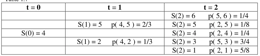
Here we perform a discrete scheme to illustrate numerical calculations needed to establish the price of this exotic instrument. Let Kc = 0.6, Tc = 1, K = 3, T = 2. The

Table 1.7

t = 0 t = 1 t = 2

S(2) = 6 p( 5, 6 ) = 1/4 S(1) = 5 p( 4, 5 ) = 2/3 S(2) = 5 p( 2, 5 ) = 1/8

S(0) = 4 S(2) = 4 p( 2, 4 ) = 1/4

S(1) = 2 p( 4, 2 ) = 1/3 S(2) = 3 p( 5, 3 ) = 3/4 S(2) = 1 p( 2, 1 ) = 5/8

represent evolution of the underlying security price over three periods of time t = 0, 1, and 2, along with the correspondent transition probabilities. From the table one can see that the security price at time 0 is $4, then at time 1 it can be either $5 or $2 with

probabilities 2/3 and 1/3 respectively. At the event S (1) = 5 security can go either to the state $6 with probability 1/4 or to the state $3 with probability ¾. If at date t = 1, S (1) = $2 then security can move either to $5, $4, $1 with transition probabilities 1/8, 1/4, 5/8 respectively. All transitions from one state to the other are assumed to be mutually independent The problem is to establish the value of the compound call-call at date t = 0 given Kc = 0.6, Tc = 1; K = 3, T = 2. We start evaluation from the date Tc = 1.

Denote C (1; 5, 6 ) = C ( t = 1; S (1) = 5, S (2) = 6 ) the value of the plain call option at time 1, given S (1) = 5, S (2) = 6. Note that the unique opportunity to avoid arbitrage is to put C( 1; 5, 6 ) = $2.5. Indeed, underlying security return over the interval [1, 2 ] is then equal to 1.2. Therefore the option return can replicate the security return for this

particular event. Note that there is no other way to prescribe an option’s value. Indeed, the option pricing does not depend on distribution and one can admit that the probability of the event { S (1) = 5, S (2) = 6 } is close to 1 and therefore the joint chance of other states can be neglected. Then from the equation ( 6 – 3 ) / C ( 1; 5, 6 ) = 6/5 follows the established price. The same way of calculations bring us to the prices:

C ( 1; 5, 6 ) = 2.5, C ( 1; 2, 5 ) = 0.8,

C ( 1; 2, 4 ) = 0.5, C ( 1; 5, 3 ) = C ( 1; 2, 1 ) = 0.

Thus,

2.5 , when ⋅ = { S ( 0 ) = 4 , S ( 1 ) = 5 , S ( 2 ) = 6 }

0.8 , when ⋅ = { S ( 0 ) = 4 , S ( 1 ) = 2 , S ( 2 ) = 5 } (1.14) C ( 1; ⋅ ) = { 0.5 , when ⋅ = { S ( 0 ) = 4 , S ( 1 ) = 2 , S ( 2 ) = 4 }

0 , otherwise

The random variable C ( 1; ⋅ ) represents a price of the underlying plain call option at date t = 1. Note that from (14) follows that

2 , when ⋅ = { S ( 0 ) = 4 , S ( 1 ) = 5 , S ( 2 ) = 6 }

1.6 , when ⋅ = { S ( 0 ) = 4 , S ( 1 ) = 2 , S ( 2 ) = 5 } C ( 0; ⋅ ) = { 1 , when ⋅ = { S ( 0 ) = 4 , S ( 1 ) = 2 , S ( 2 ) = 4 }

0 , otherwise

$5.9/12 = $0.492 at t = 1 and exercise it at T = 2 because E C ( 2, ⋅ ) > E C ( 1, ⋅ ). The return on expected option values over [ 1, 2 ] is [ E C ( 2, ⋅ ) ] / [ E C ( 1, ⋅ ) ]. That is about $1.356 at t = 2 per $1 investment at t = 1.

The direct analysis based on the precise option pricing solution shows that average return on call option is

E [χ {S ( 2 ) > 3} × C ( 2; ⋅ )/C ( 1; ⋅ )] = [3/2.5]/6 + [2/0.8]/24 + [1/0.5]/12 = 5.25/12.

That suggests less than $1 return at t = 2 per $1 investment at t = 1. This shows that the option price will not increase in average over [ 1, 2 ].Nevertheless the option price at t = 1 that bellow than $2/3 offers increase in average value of the investment. In particular the price $5.9/12 at t = 1 looks reasonable enough. The investor’s risk associated with the event when investment return billow than 1 coincides with the probability of the event to lose all capital is

Prob { C ( 2, S ( 2 )) < 5.9/12 } = P { S ( 2 ) < 4 } = 7/24

That is about 29%.

Now let us turn back to the compound option valuation. The date Tc = 1 is the expiration

date of the compound option. The buyer of the compound call option has the right to buy

underlying plain vanilla option for $0.6. The compound payoff received at the date Tc = 1

is

$max { C ( 1 , S ( 1 ); T = 2 , K = 3 ) – 0.6 , 0 } (1.15)

Therefore at the date Tc = 1 the buyer has the right but not an obligation to pay the strike

price of $0.6 and in return to get plain call option with strike K = 3 and expiration date T = 2. Let us return to the recovery of the compound premium. From (1.15) it follows that compound payoff is

2.5 – 0.6 = 1.9 , p = 2/3 ×1/4 = 1/6 Cc ( 1, C ( Tc , S ( Tc ); T , K ); T, Kc ) = { 0.8 – 0.6 = 0.2 , p = 1/3 × 1/8 = 1/24

0 , p = 19/24

Using values Cc ( 1, S ( 1 )) we enable to establish the compound option price at date

t = 0. Indeed, the stock return over the interval [ 0 , 1 ] is either 5/4 or 2/4 with the probabilities 2/3 and 1/3 respectively. If the payoff to the compound call at Tc = 1 is

equal to 0 then the value of the compound call at date 0 is obviously equal to 0. At the event when payoff is positive the return on stock and on the compound option should be equal. Otherwise as we mentioned above one can assume that the probability of a particular stock value that exceeds the strike price is as close to 1 that we can ignore the all other values. In this case we actually arrive at deterministic stock that uniquely

establishes option price by replicating stock return. Note that continuous distributed stock can also perfectly be replicated by the option. This is the case when the lowest stock value is higher then option’s strike price.

One can see that the investor pays compound premium at date 0 than pays strike price Kc

at date 1 and in return he or she obtains the plain vanilla option that cost C ( 1, S ( 1 )) =

S ( 1 ) / S ( 0 ) χ{ C ( 1, S ( 1 )) > 0.6 } = Cc( 1, S ( 1 )) / Cc( 0, C ( 0, S ( 1 ))

If the underlying option exists on [ 0 , 1 ] then by definition

S ( 1 ) / S ( 0 ) χ{ S ( 2 )) > 3 } = C ( 1, S ( 1 ) ; 2 , 3 ) / C ( 0, S ( 0 ) ; 2 , 3 ))

and stock return on the left hand side can be replaced by the correspondent option return. The compound option premium at t = 0 in both cases is equal. Thus,

4/5 × 1.9 = $1.52, p = 1 /6

Cc ( 0 , 4 ) = {

0 , p = 19/24

Note that the average value and the standard deviation of the compound call-call option are

E Cc ( 0 , 4 ) = 1.52 × 1/6 + 0.4 × 1/24 = $0.27

standard deviation Cc ( 0 , 4 ) = $0.319

For the practical use assume that an investor pays compound premium, say $0.5 at the date 0 and the compound strike of $0.6 at the date t = 1. How to represent the buyer’s risk? Analyzing the situation we see that the only event that suggests profit is the event associated with the trajectory ⋅ = { S ( 0 ) = 4, S ( 1 ) = 5, S ( 2 ) = 6 }. Indeed, the investor pays compound premium $0.5 at date 0 and then compound strike of $0.6 at date 1 that is $1.1. In return the investor receives the assets which price at date 0 is $1.52. Therefore the positive balance is $0.42. The probability of such event is 1/6. Any other possible outcome leads to the loss. Thus, the compound option risk on the investment associates with the return that is below than 1 and therefore it coincides with the event

{ C ( 1 , S ( 1 )) / 1.1 < 1 }

The probability of such an event is 1 - P { Cc ( 1 , S ( 1 )) ≥ 1.1 } = 5/6. The average loss

of exercising a compound option price is

Expected losses = E [ Cc ( 0 , 4 ) – 1.1 ] χ { C ( 1 , S ( 1 )) < 1.1 } =

= [ ( 0.4 – 1.1 ) × 1/24 – 1.1 × 19/24 ] = – $0.9

Expected profit is

E [ Cc ( 0 , 4 ) – 1.1 ] χ { C (1 , S ( 1 )) > 1.1 } = 0.42 × 1/6 = $0.07

An important investment characteristic over [ t, T ] can serve a ratio

We call it risk-effectiveness. Then the risk-effectiveness of the compound call-call investment is ℘( 0 , 1 ) = 7.78%, that might be too low to attract an investor. Let us consider next specification of the compound option. In this case assume that underlying of the compound option is a put option. Assume for simplicity that the

security data remains the same as in the Table 7. Then underlying plain vanilla put payoff at its expiration T = 2 by definition is P ( 2, S ( 2 )) = max { K – S ( 2 ) , 0 }. Therefore

0, when S ( 2 ) = 6, 5, 4, 3

P( 2, S ( 2 ) ) = {

2, when S ( 2 ) = 1

From the equation

it follows that

0, when ⋅ = { S ( 0 ) = 4, S ( 1 ) = 5, S ( 2 ) = 6 } 0, when ⋅ = { S ( 0 ) = 4, S ( 1 ) = 2, S ( 2 ) = 5 } P ( 1, S ( 1 , )) = { 0, when ⋅ = { S ( 0 ) = 4, S ( 1 ) = 2, S ( 2 ) = 4 }

0, when ⋅ = { S ( 0 ) = 4, S ( 1 ) = 5, S ( 2 ) = 3 } 4, when ⋅ = { S ( 0 ) = 4, S ( 1 ) = 2, S ( 2 ) = 1 }

The compound call-put option payoff at Tc = 1 is then can be written as

Cp ( 1, S ( 1 )) = = max { P ( 1 , S ( 1 )) – Kp , 0 }

where Kp is assumed to be equal to Kc = 0.6. Solving the equation

for Cp ( 0, S ( 0 )) bring us to the compound call-put premium

13.6 , p = 5/24 Cp ( 0, 4 ) = {

0 , p = 19/24

The expected value of the compound call-put option price is then ECp ( 0, 4 ) = $2.83. If

an investor pays a premium of $2 at date 0 and the compound strike price of $0.6 at date 1, then the profit exists only when the outcome is { S (0) = 4, S (1) = 2, S (2) = 1 }. Thus the investment of $2.6 might only bring $13,6 and therefore result in $11 of the pure profit. The probability of this event is 5/24. The event { P ( 1, S (1) ) < Kp } represents

}

)

2

(

{

)

1

(

)

2

(

)

)

1

(

,

1

(

)

)

2

(

,

2

(

K

S

S

S

S

P

S

P

<

=

χ

}

)

)

1

(

,

1

(

{

)

0

(

)

1

(

)

)

0

(

,

0

(

)

)

1

(

,

1

(

p p

p

K

S

P

S

S

S

C

S

C

>

the risk associated with this investment. Expected losses, profit, and the profitability (1.16) are

2.6 × 19/24 = $2.06 , 11 × 5/24 = $2.29 , ℘( 0 , 1 ) = 111.17%

correspondingly. This data for the long position looks much attractive for the investor than for the call-call option.

We have studied two types of compound options, call-call and call-put. Now let us take a look at two other types: put-call and put-put options. For the put-call option we again use the same data given in the Table 1.7. Put option payoff at date Tc is

Pc ( Tc , S ( Tc )) = max { Kc – C ( Tc , S ( Tc ); T , K ) , 0 }

Bearing in mind values of the call option C ( 1, S ( 1 ); 2, 3 ) given above in (1.15) we see that

0.6 , when ⋅ = { S ( 0 ) = 4 , S ( 1 ) = 5 , S ( 2 ) = 3 } Pc ( 1, C ( 1, S ( 1 )) = { 0.6 , when ⋅ = { S ( 0 ) = 4 , S ( 1 ) = 2 , S ( 2 ) = 1 }

0.1 , when ⋅ = { S ( 0 ) = 4 , S ( 1 ) = 2 , S ( 2 ) = 4 }

0 , otherwise

where

Prob { S ( 0 ) = 4 , S ( 1 ) = 5 , S ( 2 ) = 3 } = 0.5 , Prob { S ( 0 ) = 4 , S ( 1 ) = 2 , S ( 2 ) = 1 } = 5/24, Prob { S ( 0 ) = 4 , S ( 1 ) = 2 , S ( 2 ) = 4 } = 1/12, Prob { Pc ( 1, S ( 1 )) = 0 } = 5/24

In calculating these probabilities we used the assumption that all transitions are mutually independent. Then taking into an account the equation

it follows that the put-call compound option price Pc ( 0 , 4 ) is a random variable with

distribution

values 0 0.2 0.48 1.2

probabilities 5/24 1/12 0.5 5/24

We would like to point out an interesting moment in the above calculations. One might note (14) that plain vanilla call option has the same price $0.6 for two different ways at time 1. S ( 0 ) = 4, and S ( 1 ) can be either 5 or 2 then return on the stock is different though compound put payoff along two paths holds the same value

Pc { t = 1 ; S ( 1 ) = 5 , S ( 2 ) = 3 } = Pc { t = 1 ; S ( 1 ) = 2 , S ( 2 ) = 1 } = 0.6

}

)

)

1

(

,

1

(

{

)

0

(

)

1

(

)

)

0

(

,

0

(

)

)

1

(

,

1

(

c c

c

_C

_S

_K

S

S

S

P

S

P

<

The explanation of this phenomenon is that the price C (1, S ( 1 ); 2, K ) depends on σ

-algebra F12events generated by the values of S (·) occurred over the time interval

[ 1, 2 ]. Therefore when the price C ( 1 , * ) admits the same value for two different ω is

F12– measurable. On the other hand compound put pricing depends on the values S (·)

over time interval [ 0, 1 ]. The distinction in stock return on [ 0, 1 ] results in a compound put pricing.

The expected value of the put-call compound option is about $0.51. An investor who purchases the put-call option for $0.3 at t = 0 and pays the strike price $0.6 at date t = 1 purchases put-call option contract for the total of $0.9. The chance that the price of the underlying call option at date t = 2 will be bellow than $0.9 is

P{ C ( 2, S ( 2 )) ≤ 0.9 } = P{ S ( 2 ) - 3 ≤ 0.9 } = P{ S ( 1 ) = 5 , S ( 2 ) = 3 } +

+ P{ S ( 1 ) = 2 , S ( 2 ) = 1 } = 1/2 + 5/24 = 17/24.

and the average value of the losses are 3 × 1/2 + 1 × 5/24 = $1.71.

The last compound option type is put-put option. By applying the same pricing methods for P ( 1, S ( 1 ) ) we see that the put-put payoff at Tp = 1

Pp ( 1, S ( 1 )) = max { Kp – P ( 1 , S ( 1 ) ; T , K ) , 0 }

is a random variable, where Kp = $0.6, K = $3, T = 2. Then using (1.16) and that

Pp ( 1 , P ( 1, S ( 1 )) = max { 0.6 - P ( 1 , S ( 1 )) , 0 } we see that

0,6 when ⋅ = { S ( 0 ) = 4, S ( 1 ) = 5, S ( 2 ) = 6 } 0,6 when ⋅ = { S ( 0 ) = 4, S ( 1 ) = 2, S ( 2 ) = 5 } Pp ( 1 , P ( 1, S ( 1, )) = { 0,6 when ⋅ = { S ( 0 ) = 4, S ( 1 ) = 2, S ( 2 ) = 4 }

0,6 when ⋅ = { S ( 0 ) = 4, S ( 1 ) = 5, S ( 2 ) = 3 } 0, when ⋅ = { S ( 0 ) = 4, S ( 1 ) = 2, S ( 2 ) = 1 }

Applying equation

we figure out that the compound put-put price is a random variable

0,48 when ⋅ = { S ( 0 ) = 4, S ( 1 ) = 5, S ( 2 ) = 6 } 1,2 when ⋅ = { S ( 0 ) = 4, S ( 1 ) = 2, S ( 2 ) = 5 } Pp ( 0 , 4 ) = { 1.2 when ⋅ = { S ( 0 ) = 4, S ( 1 ) = 2, S ( 2 ) = 4 }

0,48 when ⋅ = { S ( 0 ) = 4, S ( 1 ) = 5, S ( 2 ) = 3 } 0, when ⋅ = { S ( 0 ) = 4, S ( 1 ) = 2, S ( 2 ) = 1 }

with the distribution

}

)

)

1

(

,

1

(

{

)

0

(

)

1

(

)

)

0

(

,

0

(

)

)

1

(

,

1

(

p p

p

K

S

P

S

S

S

P

S

P

<

values 0 0.48 1.2

probabilities 5/24 2/3 1/8

The expected value of put-put compound option is $0.47. An investor who managed to buy put-put option say for $0.21 and paid a strike price of $0.6 at date t = 1 holds the risk 5/24 to lose complete investment.

Exotic options.

In the early 1980’s, exchanges in Amsterdam, Montreal, Philadelphia, and Chicago were traded in standardized foreign currency options. Now, currency options are available to many currencies. The Security Exchange Commission regulates the options exchanges in the US. In addition to the exchanges there is an over-the-counter market where the currency options are offered by the commercial banks and brokerage firms. Unlike the currency options traded on an exchange, these currency options are tailored to the

specific firm’s interests. The number of units, strike price desired, and expiration date can be chosen by the clients.

In this paper we discuss several types of standard and non-standard options contracts. The standard options that can be reduced to the European and American options types are sometimes referred to as plain vanilla options. The non-standard options types are

commonly called exotics and they usually divide into two main classes path-depended and path-independent. We provide a survey of some popular exotic options and simultaneously introduce their valuation.

Recall some of the main definitions. A call (put) option is a contract between two parties: buyer and a seller. It gives the holder the right to buy (sell) an asset at a stated price (strike price, exercise price) on (European) or before (American) predetermined date, called maturity (expiration date). The current option price is called option price or premium.

Let S ( T ; t , x ) be a price of an underlying asset at a future date T, T > t so that

S ( t ; t , x ) = x. Denote C ( t , x ) [ P ( t , x ) ] the call [ put ] option price at date t when S ( t ) = x. Formally a plain vanilla option contract is defined by its expiration and its payoff at the expiration date. Next we will use T as a date of expiration. Then call and put values at expiration are defined as follows:

C ( T , S ( T ) ) = max { S ( T ; t , x ) – K , 0 }

(2.1) P ( T , S ( T ) ) = max { K – S ( T ; t , x ) , 0 }

where t is a current date and x is the price of an underlying asset at t.

The problem of the option pricing is to determine the call ( put ) option price at any moment of time t before the expiration date T. It is clear that the option price does not cost anything when payoff at maturity is equal to 0, and for any particular value Ξ of the asset at expiration there is a unique value of the option contract that replicates

different values implies stochastic setting of the problem. We simplify the scheme of the pricing problem. Assume that an option can only be exercised at maturity T. Such setting can be interpreted as a two step economy. Next, we shall indicate the price adjustment for the continuous time and discuss the possibility to exercise the option prior to the

expiration date.

Let us make a comment regarding a binomial scheme that is widely used as a simplified model representing an option valuation. The main drawback of the binomial benchmark pricing is that this method prescribes the same option price that does not depend on real world states probabilities. To illustrate this inaccuracy let us consider an example. Lets say the asset price today is $2, strike price $3, and at the expiration date tomorrow the asset price is either $5 or $1. Then the binomial scheme represents the constant call option price that is independent upon distribution. Thus, the option price remains the same, constant, whether the probability of the event {asset price = $5} is 0.0001 or 0.9999. One can see that such a distribution with a high reliability can be interpreted as deterministic. In the first case the call option payoff is 0 and therefore option price must be 0. In the second case the positive payoff suggests positive call option price. This remark should suggest a critical revision of the modern derivatives pricing theory.

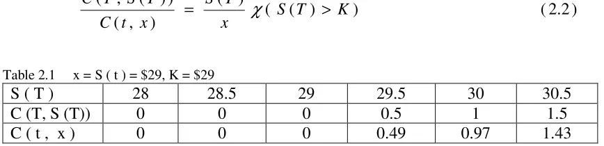
We begin with a new framework of the option pricing. The pricing problem implies the answer to the question what price should an investor pay for the option contract today given a particular payoff at the expiration?

Let an asset price today be S ( t ) = $29 and strike K = $29. If the price at maturity is S ( T ) = Q > $29, then what is the call option price today? Note that for a particular value Q at maturity there is a unique value of the option that represents an equal rate of return on stock and the option. Other possible pricing will lead us to an estimate of the option price that will be introduced bellow.

Consider the table in which the first line represents specified asset values at maturity. The values are chosen arbitrary only to illustrate the method used for

calculations. The second line of the table shows the values of the call option payoff at date T, and the third line represents current option price (premium). We use the method that suggests the same rate of return on asset and the specified valuable option

Table 2.1 x = S ( t ) = $29, K = $29

S ( T ) 28 28.5 29 29.5 30 30.5

C (T, S (T)) 0 0 0 0.5 1 1.5

C ( t , x ) 0 0 0 0.49 0.97 1.43

Though these calculations are simple algebra the only problem that makes a difference between market participants is the distribution that an investor prescribes to the values of the underlying asset. Recall that the widely popular assumption in continuous time investment sciences is that the stock price is log-normal. The accurate investigation of this assumption does not affect the problems that we are studying in this paper. Recall

) 2 . 2 ( )

) ( ( ) ( )

, (

) ) ( , (

K T S x

T S x

t C

T S T C

>

that the log-normal assumption has been commonly applied without statistically testing it. Therefore the corresponding models and parameter estimates are implied. This approach is quite popular in the investment sciences.

We begin with the option valuation. Applying (2.2), it follows that

We see that the option price is a random function. It is positive for the event when payoff of the option is positive and equal to 0 when payoff is 0. When option price is positive then the rate of return on an underlying asset and its option is the same. The possibility that the option’s payoff may be equal to 0 represents the fact that the option is a more risky financial instrument than the underlying security.

Let us consider now of a standard (plain vanilla) credit option contract. This contract’s underlying are the exchange rates between two currencies. Though the setting of the problem is quite similar to the above constructions, some peculiarities need to be specified. Let K be a strike price measured in $ / £ and q ( t ) denotes the exchange rate at time t measured in the same units. That is £1 = $ q ( t ) and therefore a £1 can be

interpreted as an asset that can be sold or bought on the $-market. All contracts are settled by delivery of the underlying currency. By definition, the contract payoff at maturity T is N max { Q ( T ) – K , 0 }, where N denotes a contract’s size. For instance, the size of a British pound call option contract traded on PLHX is N = £ 31,250. Equation (2.2) now can be rewritten in the form of:

Then the $-value of the call option contract at date t is

Formula (2.5) holds regardless; whether the currency exchange rate is stochastic or deterministic. For instance, let N = £ 31,250, K = $/ £ 1.50,

q ( T ) = $/ £1.55. Then the payoff at maturity T is equal to

£ 31,250 $/ £ ( 1.55 – 1.5 ) = $ 1,562.5

Now, let us consider the two periods in the currency exchange market where q ( t ) = K = $/ £1.50 and

qu = $1.55, pu = 0.25

} 0 , ) x , t ; T ( S -K { max ) x , t ; T ( S

x )

) T ( S , T ( P

(2.3) }

0 , K -) x , t ; T ( S { max ) x , t ; T ( S

x )

) T ( S , T ( C

= =

) 4 . 2 ( }

) ( { ) (

) ( )

) ( , (

) ) ( , (

K T q t

q T q t

q t C

T q T

C _{= χ >}

) 5 . 2 ( }

0 , )

( { max ) (

) ( $ ) ) ( ,

( q T K

T q

t q N t

q t

q ( T ) = {

qd = $1.48 pd = 0.75

The problem is to determine the call option price at the initial date t. For simplicity we define the option price related to the size N = £100 and this value could be easy replaced by an actual contract size to represent the real option’s value. Applying formula (2.5) it follows;

$4.84 pu = 0.25

C ( t , q ( t ) ) = {

0 pd = 0.75

The average and standard deviation of the option price are 1.21, and 1.815 respectively. The return on exchange rate is a random variable with a given distribution

1.0333, pu = 0.25

q ( T ) / q ( t ) = {

0.9867, pd = 0.75

for which the mean and the standard deviation are 0.9983 and 0.309 respectively. The return on a call option is equal to 1.0333 with a probability of 0.25, and 0 with a probability of 0.75. Note that the positive value of the option return coincides with the correspondent value of the return on an underlying rate of exchange. There might be a speculator who wishes to make a profit, agrees to receive 1.02% return on his investment. Then the only event that suggests this return is the event associated with the future rate qu.

Therefore the maximum price that the investor might pay for the option is $4.90 = = (qu – K ) / 1.02. The probability of the event is 0.25 that may not be enough to accept

such a deal. Indeed the average rate of return would be only 1.02 × 0.25 = 0.255. If the investor accepts 2% premium on the expected return then the upper bound of the option price is 0.25× 4.90 = $1.225. This is one simple illustration of the discrete method of the option valuation. On the other hand an investor may ask a reasonable price for the option. Ignoring real additional expenses the investor can consider the option price ($/ £)Ξ that suggests equal expected return on an option and underlying exchange rates. This setting leads to the equation

pu× [( qu – K ) / Ξ ] = pu× [ qu / q( t ) ] + pd× [ qd / q( t ) ]

The solution of the equation is Ξ = ($/ £) 0.1269.

Table 2.2

t = 0 t = 1 t = 2

q(2) = 186 p(185, 186 ) = 1/4

q(1) = 185, p(180, 185) = 2/3 q(2) = 182 p(178, 182 ) = 1/8

q(0) = 180 q(2) = 181 p(178, 181 ) = 1/4

q(1) = 178, p(180, 178) = 1/3 q(2) = 179 p(185, 179) = 3/4 q(2) = 176 p(178, 176 ) = 5/8

where p ( a, b ) represents transition probability from the state ‘a’ to state ‘b’. Assume that all transitions are mutually independent.

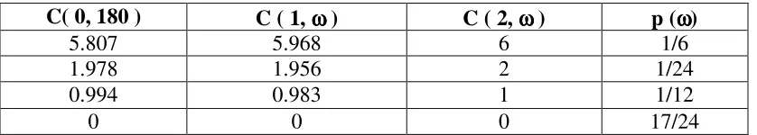
Let us consider European call option with the strike price K = ($/ £)180. We begin option price construction moving backward in time. Let us first consider the span period [ 1, 2 ]. Applying the method we used above it is easy to see that

5.968, p (180, 185, 186) = 1/6

C ( 1 , 185 ) = {

0, p (180, 185, 179) = 1/2

and

1.956, p (180, 178, 182) = 1/24

C ( 1 , 178 ) = { 0.983, p (180, 178, 181) = 1/12

0, p (180, 178, 176) = 5/24

Then

5.807, p (180, 185, 186) = 1/6

C ( 0 , 180 ) = { 1.978, p (180, 178, 182) = 1/24

0.994, p (180, 178, 181) = 1/12

0, p ( {180, 185, 179} ∪ {180, 178, 176} ) =

= 2/3 × 3/4 + 1/3 × 5/8 = 17/24

Here we denote the probability of the path {q (0) = a, q (1) = b, q (2) = c } as p (a, b, c)

and {a} ∪ {b} the union of two events ‘a’ and ‘b’. We summarize the results of these

calculations with the help of Table 2.3

Table 2.3

C( 0, 180 ) C ( 1, ωωωω ) C ( 2, ωωωω ) p (ωωωω)

5.807 5.968 6 1/6

1.978 1.956 2 1/24

0.994 0.983 1 1/12

0 0 0 17/24

finding the option price that suggests the average return of 1.015. This expected price is the solution of the equation

E C ( 1 , ω ) / 1.015 = $1.116.

Then if the investor pays $1.116 for the option, then the risk of this position is the probability

P {C (1, ω) < 1.116} = P [{C (1, ω) = 0.983} ∪ {C (1, ω) = 0}] = 1/12 + 17/24 = 19/24

This high risk results from nonsymmetrical distribution of the stochastic exchange rate. Note that in this example one can reach an arbitrary high average return on an option by choosing the option price that is sufficiently small. But the risk of any price will not be less than 17/24. We can use the data provided by Table 2.2; to determine put option price. Let us consider an European put option with the strike price of K = 182. Repeating the previous steps used for the call option valuation we arrive at

0, p (180, 185, 186) = 1/6

P ( 1 , 185 ) = {

(185/179) × 3 = 3.1001, p (180, 185, 179) = 1/2

and

0, p (180, 178, 182) = 1/24

P ( 1 , 178 ) = { (178/181) × 1 = 0.9834, p (180, 178, 181) = 1/12 (178/181) × 6 = 6.0682, p (180, 178, 176) = 5/24

Then

6.1364, p (180, 178, 176) = 5/24 P ( 0 , 180 ) = { 3.0168, p (180, 185, 179) = 1/2

0.9945 p{180, 178, 181}) = 1/12

0, p{180, 185, 186} ∪ {180, 178, 182}) = 5/24

The mean and the standard deviation of the put premium are 2.8697, 2.0598

correspondingly. Let the investor pay $1 premium for the put option. Then the risk to receive less funds than invested at expiration is 7/24. This risk is associated with the events {q (2) = 186, 182, or 181}. If an investor decides to pay $4 then the risk is P {q (2) = 186, 182, 181, 179} = 19/24.

Now let us consider the nonstandard derivative contracts. Exotic option is generic name that refers to variations of the basic options. Options are referred to as being path-independent if their payoff does not depend on the path during the life of the option. First let us examine some exotic option contracts.

Cash-or- nothing call or put options are defined by their payoff at maturity as

Ccn ( T , q ( T )) = X χ { q ( T ) > K }

Pcn ( T , q ( T )) = X χ { q ( T ) < K }

where X is a predetermined constant and q ( t ) is interpreted as the spot exchange rate in dollars per unit of foreign currency at time t, t ≤ T. Note, that in contrast to the

continuous payoff of the standard option (2.1) the cash-or-nothing options have discontinuous payoff. In contemporary financial books the cash-or nothing options are also known as digital or binary options. In this case the constant X usually assumed to be equal to 1. The valuation of options contracts follows the formula

where N is the contract size expressed in foreign currency, K is the strike price, q (T) is the currency exchange rate at date T. Let us use a numeric example. Assume that the underlying security data is given by the Table 2.2, N = X = 1. Then using the same algebra one arrives at the table

Table 2.4

Ccn ( 0, 180 ) _Ccn ( 1, ωωωω ) Ccn ( 2, ωωωω ) p (ωωωω)

0.9677 0.9946 1 1/6

0.989 0.978 1 1/24

0.9945 0.9834 1 1/12

0 0 0 17/24

Each row in the Tables 2.3 or 2.4 is the path of call option for some fixed elementary event ωo = { q (0, ωo), q (1, ωo), q (2, ωo) }, and therefore for the fixed ωo the option’s

rates of return coincide with the correspondent rates of return of the underlying exchange rate. This remark is valid for the other exotic options of the European type.

Assets-or- nothing call or put option’s payoff at maturity is defined as

Can ( T , q ( T )) = q ( T ) χ { q ( T ) > K }

Pan ( T , q ( T )) = q ( T ) χ { q ( T ) < K }

The pricing formulas can be found from the equation (2.4). Then

Can ( t , q ( t )) = q ( t ) χ { q ( T ) > K }

Pan (t , q ( t )) = q ( t ) χ { q ( T ) < K }

} )

( { )

( ) ( )

$( ) ) ( , (

) 7 . 2 ( }

) ( { )

( ) ( ) $( ) ) ( , (

K T q X T q

t q N t t

q t P

K T

q X T q

t q N t t

q t C

cn cn

< =

> =

Gapoptions are those contacts for which call payoff is defined to be

Cg ( T , q ( T )) = ( q ( T ) - R ) χ { q ( T ) > K }

where K > R. The value of the contracts can be represented by the (2.7) where X = q ( T ) – R. If K < R then payoff can be represented as

( q ( T ) - R ) χ { q ( T ) > K } = ( q ( T ) - R ) χ { K < q ( T ) ≤ R } +

+ ( q ( T ) - R ) χ { q ( T ) > R }

Note that if the buyer of the Gap call option still has the right but not an obligation to exercise option, it is clear that for a particular exchange rate such that K < q ( T ) ≤ R the investor will not exercise it. Indeed, why would the buyer pay $( K + R ) in order to receive less then invested? Thus the payoff amount is actually reduced to the standard option

( q ( T ) - R ) χ { q ( T ) > K } = ( q ( T ) - R ) χ { q ( T ) > R }

The gap-put payoff is

Pg ( T , q ( T )) = ( R - q ( T ) ) χ { q ( T ) < K }

where K < R. Then the gap-put price can be performed by the formula (2.7) where X = R – q ( T ).

Paylateroptions are defined by their payoff as follows

Cpl ( T , q ( T )) = ( q ( T ) - K - Cpl ( t , q ( t )) ) χ { q ( T ) > K }

(2.8) Ppl ( T , q ( T )) = ( K - q ( T ) - Ppl ( t , q ( t )) ) χ { q ( T ) < K }

where Cpl ( t , q ( t )) , Ppl ( t , q ( t )) are premiums to the options specified at date t and

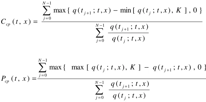
paid only on the exercise of the options. These are up-front payments paid at date t. One might think that paylater payoff can be negative. We show that it is impossible under the interpretation of the option price that is introduced in this paper. To produce the valuation of the problem let us look at benchmark formula (2.5). The solution to this equation is

The put problem solution can be represented in the similar form. Bearing in mind that the payoff of the paylater option depends on its premium, we arrive at the equation

) ) ( , ( ) (

) ( )

) ( ,

( C T q T

T q

t q t

q t

C_pl = _pl

) 9 . 2 ( } )

( { ] ) ) ( , ( )

( [ ) ( )

) ( ,

( t q t q t q T K C t q t q T K

Solving the equation for Cpl ( t , q ( T ) ) we get the call paylater option solution

Similarly,

The solution of the paylater option problem in Black-Scholes’ setting can be found for example in [7]. Their approach to the solution construction is different, therefore we make some remark to their design. In [7] the payoff of the call option was decomposed into sum of two terms

[ q ( T ) - K ] χ (q ( T ) > K ) - Xcχ (q ( T ) > K )

where Xc is an unknown constant. The first term then was interpreted as the ordinary

option payoff. Though the value Xc was considered as a constant, the second term was

interpreted as the binary option payoff with the option premium Xc. Bearing in mind this

interpretation the value Xc + K was interpreted as the paylater option premium. It is easy

to see that the correctness of this decomposition is doubtful as far as Xc relates to paylater

option and not to the cash-or-nothing option. Furthermore, Xc is not a constant it by

payoff definition is an unknown function in t.

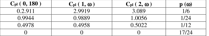
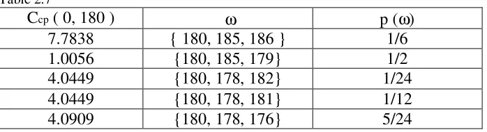
In the Table 2.5 we enclose the valuation of the paylater call option, when underlying is the value of foreign currency unit. Its value is given in Table 2.2.

Table 2.5

Cpl ( 0, 180 ) Cpl ( 1, ωωωω ) Cpl ( 2, ωωωω ) p (ωωωω)

0.2.911 2.9919 3.089 1/6

0.9944 0.9889 1.0056 1/24

0.4978 0.4958 0.5022 1/12

0 0 0 17/24

Indeed, applying the formula (2.10′) we see that

[185 / (185 + 186)] (186 – 180) = 2.9919, p = 1/4 × 2/3 = 1/6 C ( 1, 185 ) = {

0, p = 3/4 × 2/3 = 1/2,

} ) ( { ] ) ( [ ) ( ) (

) ( }

) ( { ]

) ' 10 . 2 ( )

( [ ) ( } ) ( { ) (

) ( )

) ( , (

K T q K T q T q t q

t q K

T q K

T q T q K T q t q

t q t

q t C_pl

> −

+ = >

−

− +

> =

χ χ

χ

) ' ' 10 . 2 ( }

) ( { ] ) ( [

) ( ) (

) ( )

) ( ,

( K q T q T K

T q t q

t q t

q t

P_pl − >

+

[ 178 / (178 +182 )] ( 182 – 180) = 0.9889, p = 1/8 × 1/3 = 1/24

C ( 1, 178 ) = { [ 178 / (178 +181 )] ( 181 – 180) = 0.4958, p = 1/4 × 1/3 = 1/12

0, p = 5/8 × 1/3 = 5/24,

2.9919, p = 1/6

C ( 1, 185 ) 0.9889, p = 1/24

C ( 1, q ( 1 )) = { = { 0.4958, p = 1/12

C ( 1, 178 ) 0, p = 17/24,

2.911, p = 1/6 0.9944, p = 1/24 C ( 0, q ( 0 )) = { 0.4978, p = 1/12

0, p = 17/24,

186 – 180 – 2.911 = 3.089 C (2, q ( 2 )) = [q ( 2 ) – K – C (0, 180)] χ {q ( 2 ) > K} = { 182 – 180 – 0.9944 = 1.0056

181 – 180 – 0.4978 = 0.5022 0

Note, that for the simplicity we omitted index ‘pl’ that specifies paylater option. One might see that the risk characteristics of the paylater call option as well as other exotics call option with the same strike price that have been introduced above, coincide with the correspondent risk characteristics of the standard European option with the same strike price. All these options offered the same return even though their premiums and payoffs are different.

A collar contract payoff at maturity T is defined as

I ( T ) = min { max { q ( T ) , K1 } , K 2 }}.

Note, that this payoff can be rewritten in the form

I ( T ) = K1χ { q ( T ) ≤ K1 } + q ( T ) χ { q ( T ) ≤ ( K1 , K2 ] } +

(2.11) + K2 χ { q ( T ) > K2 }

Below, we introduce the standard arguments that perform the valuation idea. Using an identity

χ { q ( T ) ≤ K} = 1 - χ { q ( T ) > K}

one can see that

Therefore,

I ( T ) = K1 - K1χ { q ( T ) > K1 } + q ( T ) χ { q ( T ) > K1 } -

- q ( T ) χ { q ( T ) > K2 } + K2 χ { q ( T ) > K2 } = K1 +

+ [ q ( T ) - K1 ] χ { q ( T ) > K1 } - [ q ( T ) - K2 ] χ { q ( T ) > K2 }

The right hand side of this equality is equal to a portfolio holding $K1 cash, long

European call with the strike price K1 , and short European call with the strike price K2.

This decomposition of the I ( T ) is not a unique representation. Indeed, it can be easily checked that

I ( T ) = K1 + K2 - q ( T ) + [ q ( T ) - K1 ] χ { q ( T ) > K1 } -

- [ K2 - q ( T ) ] χ { q ( T ) < K2 }

Thus, collar payoff is equivalent now to the value of the portfolio that contains

$( K1 + K2 ) cash, short stock, long European call, and short European put. The price of a

collar contract at any time prior to the expiration coincides with the price of the portfolio. We introduce the direct evaluation of the collar contract. From formula (2.11) it follows that collar payoff is a collection of three hypothetical financial instruments with payoffs

I1 ( T ) = K1χ { q ( T ) ≤ K1 }

I2 ( T ) = q ( T ) χ { q ( T ) ∈ ( K1 , K2 ] }

I3 ( T ) = K2χ { q ( T ) > K2 }

maturity T. Then the collar contract price at date t is I ( t ) = I1 ( t ) + I2 ( t ) + I3 ( t ) ,

where

A chooser or as-you-like option is the next exotic option type.

A holder of this option can choose whether the option is a call or a put after a specified

period of time. Consider a chooser option that matures at moment Tch , the maturity of

} )

( { ) (

) ( )

(

} ] , ( ) ( { ) ( ) (

} )

( { ) (

) ( )

(

2 2

3

2 1 2

1 1

1

K T

q T

q t q K t

I

K K T

q t

q t I

K T

q T

q t q K t

I

> =

∈ =

≤ =

χ χ

the underlying call and put denote Tc , Tp respectively. Here min (Tc , Tp ) > Tch . Thus,

the values of underlying call and put at date Tch are C ( Tch , q (Tch ) ; Tc , Kc ) ,

P ( Tch , q (Tch ) ; Tp, Kp ); where q ( t ) is the call and a put deliverable security, and K

with subscript c and p as correspondent strike prices. To start evaluation of the chooser option it is necessary to establish payoff to the option. The payoff to the chooser option is

co (Tch , q (Tch )) = max { C ( Tch , q (Tch ) ; Tc , Kc ) , P ( Tch , q (Tch ) ; Tp, Kp ) }

Then

Note that:

C (Tch , q ( Tch ); Tc , Kc )) χ { C ( Tch , q (Tch ) ; Tc , Kc ) ≥ P ( Tch , q (Tch ) ; Tp, Kp ) } =

= C (Tch , q ( Tch ) ; Tc , Kc )) χ { q ( Tc ) > Kc },

P (Tch , q ( Tch ) ; Tp , Kp )) χ { C ( Tch , q (Tch ) ; Tc , Kc ) < P ( Tch , q (Tch ) ; Tp, Kp ) } =

= P (Tch , q ( Tch ) ; Tp , Kp )) χ { q ( Tp ) < Kp , q ( Tc ) < Kc }

Therefore,