Hybrid Algorithm for Optimization Problems Applied to
Single Machine Scheduling
Hemmak Allaoua
Computer Science Department University of Bejaia, 06000 Bejaia,
Algeria
Bouderah Brahim
Department of Computer Science Laboratory of Pure and Applied Mathematics
University of M’sila, Algeria
ABSTRACT
In this paper, we will present a new variant of genetic algorithm to solve optimization problems where the number of feasible solutions is very important. This approach consists on a hybrid algorithm between genetic algorithms introduced by J. Holland (1975) and dynamic programming method of R. Bellman (1957). Then we will apply this hybrid algorithm to solve a single machine scheduling problem that consists to minimizing the sum of earliness and tardiness costs with common due date. Our goal is designing a new approach to find a good near solutions for combinatory problems as scheduling problems or traveling salesman problem which have an exponential number of solutions and known as NP-hard problems.
Keywords
Genetic Algorithm, Scheduling, Dynamic programming, Optimization.
1.
INTRODUCTION
In the recent years, the meta-heuristics become very important and have received significant attention for solving optimization problems because they can give near solutions to combinatorial problems in reasonable time even for the biggest size problems, on the other hand, the exact methods (such as complete enumeration, dynamic programming or branch and bound methods) need a considerable time to find an optimal solution especially for big size problems. However, the approach formulation and the choice of the meta-heuristic parameters can considerably affect the quality of the results. Our approach is based on this idea, since we will develop a variant of genetic algorithm where we will adjust the parameters and use the famous principle of dynamic programming to obtain best results as possible for combinatorial problems. To show the efficiency of the approach, we will apply it on a single machine scheduling that consists to minimizing the sum of earliness tardiness costs with common due date. Our new approach is presented in Section 4. The computational results using the Benchmark instances of Biskup and Feld- mann’s (2001) are presented in Section3. Finally we could with directions and further research in Section 4.
2.
GENETIC ALGORITHM (GA)
Genetic algorithms, introduced by J. Holland (1975), are inspired from the Darwin evolution theory: in the population evolution, the best individuals, which are more adapted to their environment, can outlive for a long time, on the on other hand, the individuals which are not fits to their environment disappear with the passage of generations. So, each individual is coded by its chromosome and a fitness function to be defined to evaluate individuals. Firstly, GA consists to randomly generate initial population, then, genetic operators (selection, crossover, mutation), within specified probabilities, are applied to produce a new generation which considered best than its previous. This
process must be iterative for a great number of generations as shown in the algorithm follow:
Begin
Initialization; Repeat Evaluation; Selection; Crossover; Mutation;
Until (Criteria Stopping); End.
However, the individuals encoding, fitness function, selection method, probability crossover, probability mutation and criteria stopping depend of the treated problem, so they must be carefully (empirically) chosen and can considerably improve the solution quality.
3.
DYNAMIC PROGRAMMING (DP)
Dynamic programming method, introduced by R. Bellman (1957), is based on his famous theory: “every optimal policy is composed of optimal sub policies”. It can be applicable to solve sequential combinatorial problems (as the most problems are) by breaking them down into simpler steps. Since, we must express the objective of the (k+1) order sub problem in function of the objective of the k order sub problem. So, the last problem order will represent the entire problem proposed. This relation is called bellman equation. When applicable, the method takes much less time than naive methods and it obtains exact solution but it stay costly in time (exponential time complexity), for this, it’s discouraged for biggest size problems.
However, we will not use exactly this approach, but we will inspire the idea that we let the size of the problem increase progressively within the generations. Since, at each iteration, only the best solutions outlive.
4.
PROPOSED META-HEURISTIC:
HYBRID ALGORITHM (HA)
The HA that we will present consists at genetic algorithm where the size of the treated problem crow within the generations such as in the evolution theory. That s mean, in the population generations, the problem of the generation k must be “less” than the one of generation n. As well as, when we apply the GA, only the best individuals will stay in the population. The algorithm start with an initial problem size n0, then, the size nk will crow with the passage of generations:
nk = n0 + [current_iteration*nbr_iterations / n ]
Where:
nk: size of the problem at the current generation;
n: size of the entire problem;
current_iteration: current generation order;
nbr_iterations: total number of generations;
[x]: entire part of x;
4.1
PROBLEM PRESENTATION
To show our approach efficiency, we will applied it on a single machine scheduling problem of independent jobs where the objective consists to minimize the sum of earliness and tardiness penalties against common due date. This problem was treated in many search subjects where was proofed as NP-hard problem and was applied in JIT (Just-In-Time) philosophy as in manufactures, commerce, transport, …
4.2
Notation
I : a set of n jobs: I = 1 , 2 , …. , n ; d : common due date of all the n jobs ; Ci : complete time of job i ;
pi : processing time of job i ;
Ei = max{d-Ci , 0} (Earliness of job i)
Ti = max {Ci-d , 0} (Tardiness of job i)
i : penalty per unit time of earliness for job i ;
i : penalty per unit time of tardiness for job i ;h : parameter of common due date : d = h * T ; where:
nk
p
iT
1 ; h
0.2 , 0.4,0.6,0.8
.4.3
Statement
n independent jobs to be processed on a single machine without interruption with common due date d;
Each job is available at time 0;
Each job must be processed just once;
For each job i, the processing time pi , the cost per unit time of
earliness i the cost per unit time of tardiness i are given and
assumed integer;
The objective is:
n
k1
(
iE
i iT
i)
min
.4.4
Literature
In the recent years, this type of problems has received significant attention and become important with the advent Just-In-Time (JIT) concept, where early and tardy deliveries are highly discouraged. For example, the just-in-time-principle states that the right mount of goods should be produced or delivered at exactly the right time. According our search, we have found the pioneers studying of this type of problems: Kanet (1981) [6] [8], Lee and Kim (1995) [1], James (1997), Gordon et al. (2002) [4], Feldmann et Biskup (2003) [1] [2] [3], Hino, Ronconi et Mendes (2005) [7], Lin, Chou, Ying (2005), Biskup and Cheng (1999) [9], Hall and Posner (1991) [5]. On the other hand, some work has been done on solving this type of problem by exact methods. [17] [18] [20]. Other searchers have treated heuristics methods. [10] [11] [13] [16] [19] [22]. Some works used genetic algorithm as meta heuristic. [14] [21] [23]. We note that the problem has treated in many options: single machine [1] [15] [20] [22], two machines [10] and multi machines [11] [12].
4.5
Problem properties
For this problem, an optimal solution must satisfying three optimality properties. To obtain the objective value more
efficiently, these three properties are integrated in our meta-heuristic.
Property 1
. An optimal schedule does not contain any idle time between any consecutive jobs.Property 2
. An optimal schedule is V-shaped around the common due date: the jobs complete before or on the common due date are sorted in decreasing order of the ratios pi/αi, and the jobs starting on or after the common due date are sorted in increasing order of the ratios pi/βi.P
roperty 3.
In the optimal schedule, either the first job starts at time zero or the completion time of one job coincides with the common due date.These properties can be established using proof by contradiction. Kanet (1981), Lee and Kim (1995), Gordon et al. (2002), Feldmann et Biskup (2003), Chou, Ying (2005), Biskup and Cheng (1999), Hall and Posner (1991).
4.6
Encoding
Traditionally, candidate solutions or individuals (also called phenotypes) are represented in binary as strings of 0s and 1s, but other encodings are also possible. Those abstract representations are called chromosomes or genotypes of individuals. However, in our case, a chromosome (feasible solution) consists on an array of (n+1) integer numbers, the first element represents the beginning time of the sequence and the other n elements represent the sequence itself. Example: the following vector encode the sequence (2,6,1,4,5,3) that beginning at time 4:
So, a population of m individuals will be represented by a matrix m*(n+1), with the passage of generations, this matrix will crow against two dimensions: its width (the problem size) and height (the generation size).
4.7
Fitness function
The fitness function is defined over the genetic representation and measures the quality of the represented solutions. It is always problem dependent. An ideal fitness function correlates closely with the algorithm's goal, and yet may be computed quickly. However, it must not favorite some solutions that may converge quickly toward a local maximum. In the other hand, fitness function is to maximize, since the best solutions may have a greater value of fitness function. So, it may be inversely proportional to the objective (because the objective is to maximize). Many processes are possible to adjust the fitness function, in the first hand, to prevent premature convergence or diversity, in the other hand, to assure uniform repartition of the solution. The linearization and exponentiation are used in this way. So, for these reasons, we have used the following rule of fitness:
Fitness(x) = h * (1-obj(x)/sum_obj)0.1+1. Where h is the common due date rate, x is a chromosome, solution (individual of the population) and obj(x) the value of its objective function. Our experimental results show that this rule produces good results.
4.8
Initialization
Initially many individual solutions are randomly generated to form an initial population. Traditionally, uniform law probability must be used to cover all space solutions (space search). So, that prevents the algorithm to prematurely
converge to a local optimum. The initial population size depends on the nature of the problem. Occasionally, the solutions may be "seeded" in areas where optimal solutions are likely to be found. For our case, we have chosen gen_size0 = 256 and this number will crow at each iteration, with a rate that as every natural population evolution. In fact, this is the essential difference between the genetic algorithms family and our variant, because, in any evolutionary phenomenal , the size of the populations crow with the passage of the populations.
4.9
Evaluation
This step consists to compute the objective for each individual then its fitness. Also, it computes the minimum of objectives values and save the solution corresponding. So, at the last iteration, this step allow us to obtain the best individual of the population, it is the near optimal solution searched.
4.10
Selection
This step consists to select which individuals are fits to participate for producing the next generation. Individual solutions are selected through a fitness-based process, where fitter solutions (as measured by a fitness function) are typically more likely to be selected. Certain selection methods rate the fitness of each solution and preferentially select the best solutions. Other methods rate only a random sample of the population, as this process may be very time-consuming. We have opted for fortune wheel method where the individual having a great fitness, is probable to be selected using the following implementation:
Function roulette() As Integer Dim i As Integer Dim r, s1 As Double s = 0
Randomize()
r = Rnd() * sum_fitness i = 0
While s < r i = i + 1 s = s + fitness(i) End While
roulette = i End Function
The crossover allows producing new child solutions from couples of parent solutions. For each new couple of child solutions to be produced, a couple of parent solutions is selected for breeding from the pool selected previously as shown as follow:
Parent 1 4 2 6 1 4 5 3
Parent 2 0 1 4 2 3 6 5
Crossover
Child 1 4 6 4 2 3 5 1
Child 2 0 2 6 1 4 3 5
This crossover operator is called 2 points crossover. The two points are randomly chosen, but, for good efficiency, the first point is chosen before the common due date d, the second point after. According the experimental results, we have obtain a best results with crossover probability pc = 0.75.
4.11
Mutation
The mutation genetic operator consists to give just small modification at the child obtained by crossover, that is for introduce into the population a new characters which does not exist among its parents to assure diversity in solutions space. So, that will extend the next generation to eventual good elements. In our case, in the mutation genetic operator, two jobs will be switched with a mutation probability pm= 0.01 as shown as follow:
Child k 0 3 4 2 1 6 5
Mutation
Child k 0 3 6 2 1 4 5
The switched jobs are chosen randomly but, as in crossover operator, the first one before the common due date d, the second after d, otherwise, this mutation will have any effect against the solution because the property 2.
4.12
Termination
There are many forms of criteria stopping: - Fixed number of iterations reached; - Fixed time computing;
- Solution not improved during given number of iterations;
- Optimal solution is found;
For our case, we have used a fixed number of iterations but proportional toward the problem size.
5.
COMPUTATIONAL ANALYSIS
The set of problems tested was selected from Biskup and Feldmann (2001,2003), with seven different instance sizes with n = 10; 20; 50;100; 200; 500;1000 jobs and 4 restrictive factors h = 0.2; 0.4; 0.6; and 0.8. They are used to determine the common due date, d, by multiplying the total sum of all processing times, as follows: d = h * T ; There are 10 instances for each problem size for our computational results.
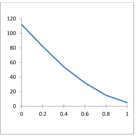
Firstly, we have computed the exact solutions for smaller sizes such as n = 5; 10 ; 20 ; 50 by using dynamic programming method then by using the proposed approach. Thus, we have obtained two solutions for each instance the one is exact solution ES and the other is near solution NS. We have remarked that the deviation = NS – NE is inversely proportional to h as shown below (see figure 1). This variation of means that when h is small; there are only few choices to schedule jobs because of their time processing pi since, some jobs can not scheduled before common due
Fig. 1 : variation of as a function of h
[image:4.595.316.557.80.141.2]Then, we have chosen the most restrictive set of 140 instances, i.e. with h = 0.2 and h = 0.4. In order to measure the effectiveness of the results obtained, we computed the average percentage deviation of the average of our solution values (H) of every 10 instances over the average of the corresponding benchmark values provided by Biskup and Feldman as follows: RP D = {(H − BF )/BF }* 100. Our results were obtained with following number of iterations numbers: 500 iterations for n= 10, 20, 50 jobs; 1000 iterations for n = 100, 200 jobs, 10000 iterations for n = 500, 1000 jobs to terminate the algorithm. The algorithm was coded in visual basic 6, VB6, an run on an PC with an Intel dual core 2.16 GHZ, 2 GB RAM.
Table 1. Percentage deviation of the average solutions
h=0.2 n=10 n=20 n=50 n=100 n=200 n=500 n=1000
BFA 1674.4 6429.2 37583.7 141143. 3
543591. 2
3348405. 6
13293514.6
HA 1674.4 6204.7 35505.1 133021. 7
509500. 7
3147715. 8
9208717.2
RPD% 0 -3.62 -5.85 -6.11 -6.69 -6.38 -44.36 h=0.4 n=10 n=20 n=50 n=100 n=200 n=500 n=1000
BFA 973.1 3703.7 21419.5 82120.2 315312. 9
1917425. 8
7651046.5
HA 973.1 3651.1 20519 79051.7 307061. 2
1787201. 8
7320456.9
RPD% 0 -1.44 -4.39 -3.88 -2.69 -7.29 -4.52
The computational results reported in the Table 1 above show that our algorithm improves the average of all instances. The overall average improvement for h = 0.2 is around -10.43% while it is −6.94% for h = 0.4. The CPU time in second are reported for the above obtained results.
Table 2. CPU time in Seconds
n 10 20 50 100 200 500
Time (s) for h=0.2 6 s 6 s 14 s 61 s 216 s 3325 s
Time (s) for h=0.4 6 s 6 s 14 s 59 s 212 s 3287 s
To show the complexity of our algorithm; we have also compared between the time processing in our approach and in the exact method (dynamic programming). As it is shown in table 2, our approach has polynomial complexity against dynamic programming which has exponential complexity.
6.
CONCLUSION
A new genetic algorithm was developed. It is based on the concept of dynamic programming where the population size and the chromosome of the solution are increased as the iteration number increases. The computational results are very encouraging. The authors are currently attempting to solve the other 140 remaining instances of lower restriction factors as well as comparing with the most developed meta-heuristics we have recently found in the literature. We consider that the adjusting of the approach parameters as crossover probability, mutation probability, initial population, selection method, increasing step of the population size can more improve the results. Also, we suggest extending our study by Applying it on other problems such shortest path or travelling salesman problem.
7. REFERENCES
[1]. M. Feldman, and D. Biskup, “Single-machine scheduling for minimizing earliness and tardiness penalties by meat-heuristic approaches”, Computer & Industrial Engineering, 44 (2003) 307-323.
[2]. M. Feldman, and D. Biskup, “Benchmarks for scheduling on a single machine against restrictive and unrestrictive common due dates”, Computer & Industrial Engineering, 28 (2001) 787-801.
[3]. M. Feldman, and D. Biskup, “Benchmarks for scheduling on a single machine against restrictive and unrestrictive common due dates”, Computer & Industrial Engineering, 28 (2001) 787-801.
[4]. R. Hassin, and M. Shani, “Machine scheduling with earliness and tardiness and non-execution penalties”, Computer & Industrial Engineering, 32 (2005) 683-705.
[5]. G. Li, “Single machine earliness and tardiness scheduling”, European Journal of Operational Research, 96 (1997) 546-558.
[6]. S. W. Lin, S. Y. Chou and K. C. Ying, “A sequential exchange approach for minimizing earliness-tardiness penalties of single machine scheduling with a common due date”, European Journal of Operational Research, xx Volume 177, Issue 2, Pages 1294–1301.
[7]. C. M. Hino, D. P. Ronconi, A. B. Mendes, “Minimizing earliness and tardiness penalties in a single machine problem with a common due date ”, European Journal of Operational Research, 160 (2005) 190-201.
[8]. K. R. Baker, G. D. Scudder, “Scheduling with earliness and tardiness penalties: a review”, European Journal of Operational Research, 160 (2005) 190-201.
0 20 40 60 80 100 120
[image:4.595.54.290.484.694.2][9]. T. Vallée, and M. Yiltizogli, “Présentation des algorithmes génétiques et leurs applications en économie”, Mai 2004, V .5.
[10]. C.S. Sung, J.I. Min. “Scheduling in a two-machine flow shop with batch processing machine(s) for earliness/tardiness measure under a common due date”. European J. Oper. Res., 131 (2001), pp. 95–106
[11]. J. Bank, F. Werner. “Heuristic algorithms for unrelated parallel machine scheduling with a common due date, release dates, and linear earliness and tardiness penalties”. Mathl. Comput. Modelling, 33 (4/5) (2001), pp. 363–383.
[12]. H. Sun, G. Wang. “Parallel machine earliness and tardiness scheduling with proportional weights”. Comput. Oper. Res., 30 (2003), pp. 801–808.
[13]. Ching-Jong Liao, Che-Ching Cheng. “A variable neighborhood search for minimizing single machine weighted earliness and tardiness with common due date”. Computers & Industrial Engineering. Volume 52, Issue 4, May 2007, Pages 404–413.
[14]. Liu Min, Wu Cheng. “Genetic algorithms for the optimal common due date assignment and the optimal scheduling policy in parallel machine earliness/tardiness scheduling problems”. Robotics and Computer-Integrated Manufacturing. Volume 22, Issue 4, August 2006, Pages 279–287
[15]. Bülbül, K., Kaminsky, P., Yano, C.: “Preemption in single machine earliness/tardiness scheduling”. Journal of Scheduling 10, 271–292 (2007).
[16]. Detienne, B., Pinson, E., Rivreau., D.: “Lagrangian domain reductions for the single machine
earliness-tardiness problem with release dates”, European Journal of Operational Research 201, 45–54 (2010).
[17]. Sourd, F., Kedad-Sidhoum, S., “A faster branch-and- bound algorithm for the earliness-tardiness scheduling problem”, Journal of Scheduling 11, 49–58 (2008).
[18]. Sourd, F., “New exact algorithms for one-machine earliness-tardiness scheduling”. INFORMS Journal on Computing 21, 167–175 (2009).
[19]. Yau, H., Pan, Y., Shi, L., “New solution approaches to the general single machine earliness tardiness problem”. IEEE Transactions on Automation Science and Engineering 5, 349–360 (2008).
[20]. Débora P. Ronconi; Márcio S. Kawamura , "The single machine earliness and tardiness scheduling problem: lower bounds and a branch-and-bound algorithm”, Comput. Appl. Math. vol.29 no.2 São Carlos June 2010.
[21]. S. Webster, D. Jog & A. Gupta, “A genetic algorithm for scheduling job families on a single machine with arbitrary earliness/tardiness penalties and an unrestricted common due date”, International Journal of Production Research. Volume 36, Issue 9, pp. 2543-2551, 1998.
[22]. Shih-Hsin Chen, Min-Chih Chen, Pei-Chann Chang, and Yuh-Min Chen, “EA/G-GA for Single Machine Scheduling Problems with Earliness/Tardiness Costs", Entropy 2011, 13, 1152-1169; doi:10.3390/e13061152.