Model Checking BRS based AADL Specification
Nadira Benlahrache
Department of Computer Science, Mentouri UniversityConstantine, Algeria
Faiza Belala
Department of Computer Science, Mentouri UniversityConstantine, Algeria
Taha A. Cherfia
Department of Computer Science, Mentouri UniversityConstantine, Algeria
ABSTRACT
Although the architecture description language AADL differs from other ADLs by its possibility to describe both hardware and software aspects of a system, it does not provide a formal notation for describing the deployment operation which is crucial in systems where hardware and software components are tightly coupled such as embedded systems. In this paper, we show the relevance of bigraphical reactive systems (BRS) to formalize the deployment operation of AADL architectures. The proposed approach allows, firstly a formal description of the two structures of AADL architectures, namely the platform and the application scenario, and secondly a natural modelization of the installation and the reconfiguration of AADL specification thanks to composition and transformaton operations of BRS. To validate the obtained model, we use a model checker dedicated to BRS.
General Terms
Software architecture, deployment, formal specification, ADL.
Keywords
Architecture language, bigraphs, BRS, installation, reconfiguration.
1.
INTRODUCTION
The architecture description languages (ADLs) [1] have been defined to precisely specify a software architecture consisting primarily of functional components described in terms of their behaviour, interfaces and interconnections. The existing ADLs often have a specific characteristics related to their motivation, their use and possibly the associated formal semantics [2]. Due to the increasing complexity of the hardware/software components interactions, these languages become difficult to use in some aspects of the development cycle of software systems, especially the specification of deployment mechanisms and reconfiguration. In fact, the deployment specification of software architecture is usually "mistreated" despite that the consistency of the operation of installing software entities on those of hardware type [3], must be ensured for designing applications.
AADL language is a standard promoted by the SAE [4] for analysis and design of the software application. It is able to convey within a single notation all information concerning the organization of the application and its runtime platform. Therefore, it combines the abstract and the concrete aspects of a software specification. Several tools are proposed around this language, such as Osate [5] and Ocarina [6], etc.
Moreover, bigraphical reactive systems (BRS) introduced in [7] are a graphical model that can formally specify distributed applications with mobile code. They unify in a single model the two dimensions: interaction and spatial distribution [4].
In some previous works [8], authors show the relevance of this formalism to specify architectural styles and some of their relevant operations (reconfiguration, style conformance, etc). In this work we extend the use of BRS to specify deployment tasks declared in an AADL specification. Firstly, we give bigraphical formalization of the two structures: software application and runtime platform. Secondly, we define the installation and the reconfiguration tasks by respectively, a bigraphical composition and a transformation one. Finally, we prove the correctness of the proposed models by using a model checker for bigraphs [9].
This paper is organized as follows: we introduce in the next section the AADL language via an illustrative example. Section 3 is dedicated to the presentation of BRS. In Section 4, we give the formal description of the two AADL architecture structures, namely the platform and the application scenario. We exploit, in Section 5, our proposed BRS based model to specify the installation and reconfiguration operations thanks to the composition and transformation operations on bigraphs. Section 6 is devoted to present the validation of our model by using a model Checker tool. Finally, a conclusion will summarize our contribution and give some perspectives for a future work.
2.
PRESENTATION OF AADL
LANGUAGE
AADL (Architecture Analysis & Design Language) [4] is a language for describing software architecture with a rich vocabulary and expressive capabilities. AADL description is a set of component declarations that can be instantiated to form the architectural description. This description can be enriched through properties for functional and non-functional aspects of a software system. Property declaration allows the expression of user requirements, deployment settings and system reconfiguration. Many tools have been developed around AADL language, such as Osate [5], Topcased [10] and Ocarina [6]. They can edit AADL architectures; build the application software system from an AADL description (Ocarina) or achieving various tests (Osate, Cheddar, etc.). To present the basic architectural elements of this language, we consider a simple example expressing a communication between two threads (see tab.1).
represent its operational states. The implementation The_system.impl (tab.1) is a possible implementation of the component The_system. Table 2 shows the declaration of sub-components involved in this example.
Table 1. Example of an AADL specification.
system The_system
end The_system ;
system implementation The_system.impl
subcomponents
the_processor : processor Processor1.impl; the_process : process Process1.impl; the_memory : memory Memory1.impl; the_bus : bus Bus1.impl;
properties
Actual_Memory_Binding => reference the_memory applies to the_process;
Actual_Processor_Binding => reference the_processor
applies to the_process.thr_S;
Actual_Processor_Binding => reference the_processor
applies to the_process.thr_R;
Actual_Connection_Binding => reference the_bus applies to the_process.cnx;
[image:2.595.49.287.167.565.2]end The_system.impl;
Table 2. AADL specification of “The_system”
subcomponents.
process Process1
end Process1 ;
process implementation
Process1.impl
subcomponents thr_S : thread
ThreadSender.impl ; thr_R : thread
ThreadReceiver.impl ;
connections
cnx : event port thr_S.outPort -> thr_R.inPort ;
end Process1.impl ;
Processor Processor1
features
busAcc : requires bus access
Bus1.impl ;
end Processor1 ;
Processor implementation
Processor1.impl
subcomponents
mem : memory Memory1.impl ;
properties
Scheduling_Protocol => ( RMS );
end Processor1.impl ;
memory Memory1
end Memory1; memory implementation
Memory1.impl
end Memory1.impl;
bus Bus1
end Bus1;
bus implementation Bus1.impl
properties
Propagation_Delay => 5ms.. 7ms;
end Bus1.impl ;
AADL configuration represents a graph of components and connections. Moreover, AADL specifications (see tab.2) define implementation details of the hardware components (the_processor, the_memory and the_bus). The properties bring more details on the operational aspects of these components. In the AADL declaration of tab.2, software component the_process consists of two subcomponents of thread type, thr_S (Sender) and thr_R (receiver). These threads interact through a connection cnx, defined between the event ports: Inport and Outport (tab. 2). Other implementation details of threads, contained in the process, are given by properties such as Period and Execution time (see tab. 3).
Table 3. A thread Description.
Thread ThreadSender
features
outPort : out event port;
end ThreadSender ;
thread implementation ThreadSender.impl
properties
Period => 120ms;
Compute_Execution_Time => 30ms .. 40ms; Dispatch_Protocol => ( Periodic );
end ThreadSender.impl;
Tools developed around AADL [6, 8] give the possibility to specify AADL architecture from components involved in an AADL model. But, they do not offer a complete graphical view of an operational system instance (hierarchy of components). Also, connections and relationships between software components and hardware ones are not considered in these tools notations.
3.
INTRODUCTION TO BRS
The bigraphical theory of reactive systems (BRS) defined in [7] is based on a graphical model for the specification of distributed applications with mobile code. This model supports the two dimensions: interaction and spatial distribution of the application. It merges two types of graphs: places graph and links graph (where the name of Bigraph). Some works in literature have shown that bigraphs form a unifying framework for concurrency and mobile models, such as CCS, the π-calculus, the ubiquitous systems or Petri nets [7, 11].
3.1.
Basic Concepts
On the basis of a common set of nodes representing the physical or virtual entities of a distributed application, a bigraph is formed of two independent structures: the places graph, having the structure of a forest that shows the spatial distribution of the application, the links graph is an hypergraph establishing the model of connectivity between various nodes [11]. While an arc in the places graph shows the relationship of spaces between the nested elements of the application, an arc in the graph links establishes a connection between the ports of these elements. The two structures are orthogonal, so links between nodes can cross locality boundaries. Each tree in the places graph represents a region of space that can contain sites, corresponding to the leaves of the tree, and where other bigraphs can be hosted.
A bigraph can interact with its environment through his interfaces designed by 𝐼=𝑚,X and 𝐽=𝑛,𝑌 , where m is the number of sites in the bigraph and X the set of its inner names. Its outer interfaces are defined by n and Y which are respectively the number of regions and the set of outer-names.
Example 2: The bigraph G =(V, E, Ctrl, GP, GL) I J in Fig. 1 inspired from [12], specifies a set of users and PCs who are divided between two rooms R1 and R2. All nodes of this bigraph are defined by V
U U1, 2,U3,Pc Pc1, 2,Pc3, 1,R R2
and the set of hyper-edges or links E
L0, 1,L L2,L3,L4
1 2 2 2 32 1 2 2 3 1 2 2 4
Ctrl U : , U : , U : , Pc :2 , Pc : , Pc :2 , R : , R :
The number of sites is m = 0, i.e. no free holes in the bigraph. The bigraph contains two regions (n=2) numbered from 0 to 1 and represented by dashed rectangles, it exposes an outer name x. So its inner and outer interfaces are respectively I = <0, > and J= <2, x>.
Bigraph G = <0, > <2 ,x>
PlacesGraph GP = 02 Links Graph GL = x
Fig 1: An Example of bigraph.
3.2.
Bigraph Operations
Bigraphs may undergo many operations that make them more dynamics. Here we present, via examples, the most important ones: composition and transformation.
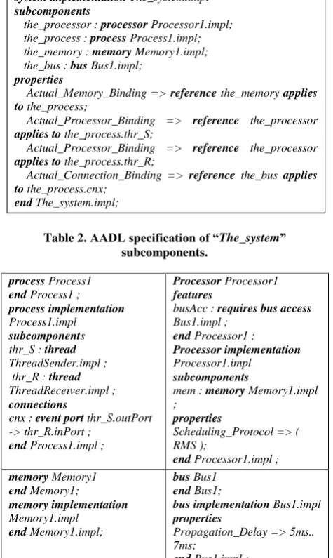
Composition: As in any graph type, the composition of bigraphs creates a new bigraph by combining two or more
bigraphs. The composition
G
H F
o
of two bigraphs F [image:3.595.332.534.74.216.2]and H is a hosting operation of bigraph F (fig.2) in the bigraph H. Thus, it is necessary that each region of F has a free site in H, i.e., there are enough free sites in H to contain all the regions of F (one site per region). The connection of the two bigraphs is achieved via a matching between outer interfaces of F with inner interfaces of H.
Fig. 2 shows how a region (bigraph F) can be hosted in a site of a contextual bigraph H.
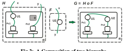
[image:3.595.47.277.153.319.2]Transformation: Two types of transformations are possible on bigraphs. The transformation of the places represents the arrival or departure of an entity. The transformation of the links, expresses the connecting or disconnecting of a node through one of its inner or outer interfaces. This dynamic is defined by a bigraph transformation rules, called Reaction Rules[11].A reaction rule is a couple of bigraphs: Redex and Reactum (before and after transformation).
Fig 2: A Composition of two bigraphs.
[image:3.595.315.542.446.509.2]A reaction rule is defined by a couple of bigraphs (R, R’) = (R: m J; R’: m’ J; µ). R is called the Redex bigraph and R' is the Reactum bigraph. µ: m’m is a correspondence between the number of sites of Redex and Reactum bigraphs.
Fig 3: Transformation of a bigraph.
The application of a rule allows identifying in the contextual bigraph, an image of the Redex bigraph, and replacing it with the Reactum one. Fig. 3 shows the effect of the application of the reaction rule (fig.3.a) on the bigraph F (fig.3.b). The result is the new bigraph F (fig.3.c).
3.3.
A Model Checker for BRS
BigMC (Bigraphical Model Checker) is a model-checker designed to operate on BRS based models [9]. The model checking in this case is achieved through an exhaustive search of all the possible states of the system specified by a BRS. The main objective of a model checking is the ability to provide a counter-example in the event that the specification is shown not to hold. This means giving the system configuration that violates the specification, and the path through the transition system by which this configuration was reached. The full grammar for BigMC bigraph terms is given as [9]:
[image:3.595.64.275.620.707.2]Table 4. BigMc terms language
M ::= E; M | E; E ::= % passive k : arity E ::= % active k : arity E ::= % rule n T T E ::= % property n P E ::= T T | T
T ::= K:T | T | T || T | $n | K | nil K ::= k [names] | k
names ::= n; names | n
n ::= [a - zA - Z][a - zA - Z0 - 9]* | -
P ::= matches(T) | terminal ()| !P
By this grammar (tab.4), we can specify all bigraph elements. M designs a BigMc model, which may be composed from other models or/and expressions (E). An expression E can be a node declaration (dynamic and arity of a given control), a reaction rule, a term (T), or a property (P). A term T can represent a single node, site or region. But also, it can be a combination of all these elements. The property P is a state definition to check with this tool. This state is achieved by applying reaction rules defined in the model according to the algorithm cited in [9]. We will use this grammar to specify our model and the BigMc to verify the specification of the installation and the reconfiguration tasks.
4.
MODELING
AN
AADL
ARCHITECTURE WITH BIGRAPHS
Several approaches in the literature adopt the concept of graphs and their transformations to model the architectural styles and their instances [8, 13], but they have not been concerned by the modelling of runtime platforms which supports the deployment of these applications. Inspired by the idea of [8], modelling software architectures by bigraphs, we have proposed in an earlier work [14] a generic formalization
.
Pc2 U
1 x
U2
Bigraph F c.
Pc1 Pc2 U1
x
U2
b. Bigraph F Reaction Rule
a R
Pc U
Pc U R’
Redex Reactum
Pc1
R
Pc1 Pc2
U1
U2 x
0
x y
y H
F
R
Pc1 Pc2
U1 U2
G = H o F
R1
Pc2 U2
R2
Pc1
x
U3
L0 L2
L4
L1
Pc3
U1
L3
0
R1
Pc1 Pc3
R2 1
R2
Pc1
0 1
Pc3 U3
L0
L1 L4
L2 L3
R1 Pc2
U2 U1
of a software architecture deployment by exploiting the operation of bigraphs composition. Our purpose here, is to continue this work and to adapt it to the description of an AADL architectural instance, which is quite rich in terms of expressiveness, but has no formal semantic definition for the deployment operation. In this section, we proceed to define a formal framework based on bigraphs, allowing firstly, modelling an AADL software application and secondly the formalization of a target environment for deployment process.
Table 5. Formalizing AADL Architectural Elements
AADL Architectural
elements Semantic in Bigraphs terms Configuration
(component system) Bigraph / Region Component (Software,
Hardware, Connector) Node
Port /Role Port / Inner-name or outer-name Interaction Port /Role Hyper-edge
Hierarchy Imbrications of Nodes / Sites Binding Properties Deployment dependencies
Mode Redex/Reactum Bigraph
Mode Transition Reaction Rule
The main elements of an AADL architectural instance, summarized in Table 5 are defined in terms of some bigraphical concepts. Each AADL component or connector of a given configuration can be formally represented by a node in a bigraph. The tree structure of the places graph maintains the hierarchy of composite components or connectors in a given AADL configuration. Moreover, the notion of control associated to a node (component or connector) is used to define interfaces of a component (ports) or those of a connector (roles) and the associated behaviors. Defined connections between ports and roles of the components (and / or connectors) are formalized by the bigraph hyper-edges. The application of these correspondence rules between AADL configuration and bigraphs concepts (Table 5) can further refine the formalization of an AADL specification which may be rather complex. So, we consider the two aspects of an AADL specification separately and attribute a couple of bigraphs for modelling the both aspects: GS and GH (s for
software, H for hardware). In AADL, all software entities that constitute the software part of the system need to be deployed on hardware components. Thus, we rely on values of the property Actual Binding to determine which software component is attached to which hardware one. The syntax of this property is as follows:
Actual_XXXX_Binding => reference to <software-component> applies to<hardware-component>.
Information analysis of this property may provide two types of information. Firstly, it helps to build separately the two bigraphs (GS and GH) corresponding to an AADL
configuration declaration and secondly to establish their relationship in terms of sites, regions and inner/outer names. The number of occurrences of this property in the AADL specification indicates the overall number of sites and regions in both bigraphs. This number can be reduced if the same hardware component name is referenced by several components of the same category. In addition, this property determines the inner-names and outer-names of bigraph. Thus, the sites represent the hardware components and regions are the software components. In our notation, a
<hardware-component> denotes a numbered site having an inner-name. Similarly, <software-component> denotes a numbered region having an outer-name. In particular, we indicate the previous two items, if they are involved by the same property, by the same label and the same number.
Obviously, if two or more elements in the same category refer to the same hardware component, they will be contained in the same region, and emit through the same hyper-edge. In our formalization approach, two AADL sub-specifications will be considered; one for the software application and the other for hardware specification supposed supporting this application. We define hence a pair of bigraphs G = (GS, GH).
The relationship between these two types of statements, expressed through properties of kind Actual…Binding is used to complete the definition of the structure of bigraph G.
Example 3: Using the example of the AADL system reported in tables 1, 2 and 3, the first bigraph GS (Fig. 4) representing
the software part of the system is deduced by applying our approach as ( ) 𝐼 𝐽 , where
VS={the_process, thr_S, thr_R, cnx } and ES = {e0, e1}. For example: vi = thr_S, ctrls(vi)= 1, prnt (thr_S)= the_process. In this scenario mS = 0, i.e. GS does not have sites, so it emits no inner-name, for this XS = . So that GS
inner interfaces are: 𝐼 〈 〉. GS outer interfaces are
defined by nS = 1 and YS = {m, c, x}. Therefore 𝐽
[image:4.595.355.505.314.516.2]〈 {𝑚 }〉.
Fig 4: Example of Bigraph GS.
Fig 5: Example of Bigraph GH.
Similarly, we attribute a bigraph GH to the AADL system description of hardware components.
The bigraph defining the target runtime platform given by an AADL declaration is ( ) 𝐼 𝐽 ,
such as: VH is a finite set of hardware components that can be nested inside each other. EH is a finite set of hyper-edges. In particularly, we focus on the parameter mH which is the number of sites, i.e. locations in the bigraph representing the availability of hardware components for the success of the software components installation. XH is the set of inner-names, which represent the interfaces of the sites.
Example 4: The bigraph in figure 5 shows the various elements of the runtime platform. The component the_memory is supposed to contain the code for a running process. A processor (the-processor) is essential to execute threads and a bus (the_bus) for the various connections. The bigraph GH in this example is given by:
- VH = {the-processor, the_memory, the_bus}. - EH = {e2, e3}.
2
1
0
x c m
the_processor the_bus
the_memory e2 e3
thr_S e0 cnx
e1
x m
-c the_process
We can identify the faces of communication ports such as: face (ctrlH (the_processeur)) = {BusAcc}, mH = 3 sites, 3 inner-names only, for this {𝑚 }. So, 𝐼
〈 {𝑚 }〉. nH =1, YH = Ф (GH contains no outer names). Therefore, 𝐽 〈 〉 and 〈 {𝑚 }〉 〈 〉.
5.
FORMALIZATION OF
INSTALLATION AND
RECONFIGURATION TASKS
Starting from the model presented above, associated to an AADL specification, we establish a formal description of software application installation on runtime platform. Besides, we associate also to the reconfiguration task a BRS-based model.
5.1. Installation Operation
The installation task is often described as a set of specific steps dictated by the software producer to install a given application on a particular platform, regarding a specific technology. This task will be defined by a composition operation of two or more bigraphs. It will be guided by the regions and sites number/labels and also by the correspondence between inner and outer names.
In order to formalize the process of installing software components on hardware ones in an AADL specification instance, we need first, to flatten the bigraph structures (both
Gs and GH). This can be justified by the fact that the
installation of subcomponents is done independently of the parent component (container).
So, for example, a decomposition of the bigraph Gs (Example 3) gives two bigraphs, one is dedicated to represent subcomponents and the other to define the context. Gs = C o Sc, where Sc is the subcomponents bigraph and C the contextual one.
Thus, according to the AADL specification, nodes and arcs of bigraph Sc can be deduced from Subcomponent and connections clauses of the container component. The added outer-name (p) (fig 6.a) indicates the new regions that can be embedded in sites having the same label. We may keep the relationship between the subcomponents and the container component.
Threads thr_S and thr_R are grouped in one region because they belong to the same sub-component category and implied by the same property (Actual binding) and also they refer to the same hardware component; the processor the_processor in our case.
[image:5.595.318.542.195.320.2]Having both bigraphs Gs and Sc (fig.6.a), it is then possible to deduce the bigraph C (fig.6.b) based on the composition principle.
Fig 6: Representation of subcomponents and contextual bigraphs.
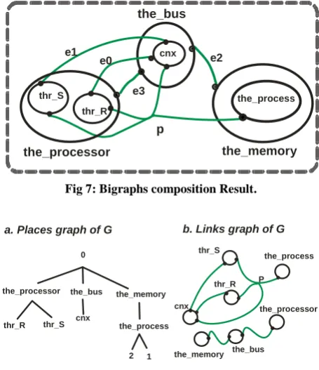
The composition of bigraphs GH and GS will be done in two
steps: G = GH o GS = GH o (C o Sc) = (GH o C) o Sc.
[image:5.595.314.542.197.461.2]Thus, the inner/outer names disappear if they are satisfied (i.e. an outer-name of a region corresponds to an inner-name of a site, both having the same label). Fig 7 illustrates how the software components will be installed on relevant hardware components. The obtained bigraph offers a mathematical model which allows the reasoning on installation task and gives the possibility to check its correctness in terms of dependencies satisfaction.
Fig 7: Bigraphs composition Result.
Fig 8: Places and links graphs of G.
Places graph (fig.8.a) shows the relationship between components after installation operation. Later and after installation task, information contained in this graph leads the reconfiguration choices.
5.2. Reconfiguration Operation
Software reconfiguration constitutes an important activity of the deployment process. At architectural level, reconfiguration of component-based system provides a set of transformations preserving some properties despite system runtime changes. Adding, removing and refining components or interaction links may be some of reconfiguration examples [15]. AADL language offers the concept of modes to represent operational, alternative and predefined states of a component or a complete system. Thus, in AADL architectural systems may be reconfigured by switching from one mode to another. In the following, we will show how BRS based models formalize architectural reconfiguration of AADL specification thanks to modes handling.
the_process
thr_R thr_S
cnx
P b. Links graph of G
the_process 0
thr_R
the_memory the_bus
a. Places graph of G
the_processor
thr_S cnx
the_processor
the_bus the_memory
2 1
the_processor
the_bus
the_memory p
e2
e3 thr_S
e0
e1 cnx
thr_R
the_process
c
x p
cnx Thr_R
0 1
a. Bigraph Sc
Thr_S
e0
e1
p
m
1 0
[image:5.595.58.271.624.693.2]Table 6. AADL Reconfiguration of “the_process”.
process Process1
features
P_ev : in event port ;
end Process1 ;
process implementation Process1.impl
subcomponents
thr_S : thread ThreadSender.impl ;
thr_R1 : thread ThreadReceiver.impl1 in modes (mode1) ; thr_R2 : thread ThreadReceiver.impl2 in modes (mode2) ;
connections
cnx1 : event port thr_S.outport -> thr_R1.inport in modes
(mode1) ;
cnx2 : event port thr_S.outport -> thr_R2.inport in modes
(mode2) ;
modes
mode1 : initial mode ; mode2 : mode ;
mode1 -[P_ev]-> mode2 ; mode2 -[P_ev]-> mode1 ;
end Process1.impl ;
thread implementation ThreadReceiver.impl1
properties
Compute_Execution_Time => 5 Ms .. 5 Ms ; Period => 10 Ms ;
end ThreadReceiver.impl1 ;
thread implementation ThreadReceiver.impl2
properties
Compute_Execution_Time => 8 Ms .. 8 Ms ; Period => 20 Ms ;
end ThreadReceiver.impl2;
We denote any system configuration by a pair (S, M) expressing the dynamic of a system S in a mode M. Reconfiguration is specified by transitions between configurations thanks to mode changes. To achieve its formalization, we exploit dynamic behavior of bigraphs. Reaction rules expressing various changes between bigraphs may be used in this context.
Definition: Given a mode transition
[(C, M)
→
(C,
M’)]
associated to an AADL component specification C, its formal semantic is defined by a reaction rule composed of two bigraphs (Redex, Reactum), noted r: (R, R') where: R: is a bigraphical model of C in mode M;
R': is a bigraphical model of C in a new mode M'.
Fig 9: Bigraphical Reconfiguration of “the_process”.
Figure 9 represents a bigraphical transformation defining the AADL reconfiguration of the_process component. The purpose of this rule is to allow the toggling of the component the_process between two different modes associated to the threads Thr_R1 and Thr_R2.
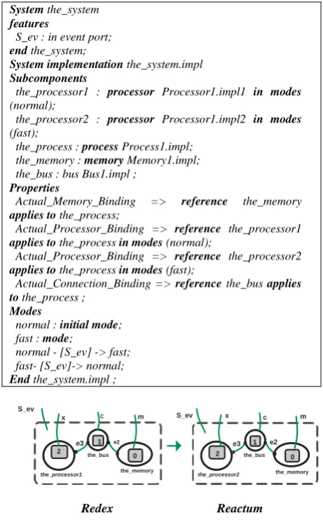
[image:6.595.313.544.138.514.2]We show in the following example (table 7, Fig. 10), how our approach is applied to manage the substitution of a processor component by a faster one, thanks to the arrival of a trigger event from “S_ev” port
.
Table 7. AADL reconfiguration of runtime platform.
System the_system
features
S_ev : in event port;
end the_system;
System implementation the_system.impl
Subcomponents
the_processor1 : processor Processor1.impl1 in modes
(normal);
the_processor2 : processor Processor1.impl2 in modes
(fast);
the_process : process Process1.impl; the_memory : memory Memory1.impl; the_bus : bus Bus1.impl ;
Properties
Actual_Memory_Binding => reference the_memory
applies to the_process;
Actual_Processor_Binding => reference the_processor1
applies to the_process in modes (normal);
Actual_Processor_Binding => reference the_processor2
applies to the_process in modes (fast);
Actual_Connection_Binding => reference the_bus applies to the_process ;
Modes
normal : initial mode; fast : mode;
normal - [S_ev] -> fast; fast- [S_ev]-> normal;
End the_system.impl ;
6.
VALIDATION WITH BIGMC
To validate our model, we use the BigMc tool [9]. It is a model checker dedicated to BRS. Checking process is based on applying reaction rules defined in the bigraphical model. In the first step, we want be sure if our model, obtained by composition and which may represent the application deployed on its runtime platform, is correct. In the second step, we will check the consistency of the reconfiguration task, expressed by reaction rules.
6.1.
Installation Checking
Table 8 summarizes our bigraphical model expressed in the appropriate grammar (of the BigMc tool). We specify some reaction rules to simulate the operation of bigraphical composition. These rules are specified exploiting disjoint bigraphs of figures 4 and 5, we obtain a new bigraph modelling the installation task.
[image:6.595.59.265.522.631.2]Redex Reactum
Fig 10: Bigraphical Reconfiguration of “the_system”.
x C m
0 1 2
the_processor1
the_bus
the_memory e2
e3
x c m
0 1 2
the_processor2
the_bus
the_memory
e2 e3 S_ev
m c thr_S cnx1
e0 e1
x
m c the_process
thr_R1
thr_S cnx2 e0
e1
x
the_process
thr_R2
S_ev
S_ev
Table 8. The model of Sender/Receiver system in BigMc
#Nodes
%active the_processor : 2; %passive thr_S : 3; %passive thr_R : 3; %active the_bus : 3; %passive cnx : 4; %active the_memory : 2; %active the_process : 2;
#Links
%name x; %name m; %name p; %name c; %name e0; %name e1; %name e2; %name e3; #Sender/Receiver model
the_processor[x,e3] | the_bus[c,e2,e3] | the_memory[m,e2] | the_process[m,-].(thr_R[x,e1,-] | thr_S[x,e0,-] | cnx[c,e0,e1,-];
#Reaction rules
the_process[m,-].(thr_R[x,e1,-] | thr_S[x,e0,-] | cnx[c,e0,e1,-])-> the_process[m,p] || (thr_R[x,e1,p] | thr_S[x,e0,p]) || cnx[c,e0,e1,p]
the_memory[m,e2].$0 || the_process[m,p] -> the_memory[-,e2].the_process[-,p].($1 | $2) || nil;
the_processor[x,e3].$2 || (thr_R[x,e1,p] | thr_S[x,e0,p]) -> the_processor[-,e3].(thr_R[-,e1,p] | thr_S[-,e0,p]) || nil; the_bus[c,e2,e3].$1 || cnx[c,e0,e1,p] -> the_bus[-,e2,e3].cnx[-,e0,e1,p] || nil;
%property consistency (the_processor[-,e3].(thr_R[-,e0,p]|thr_S[-,e1,p]) | the_bus[-,e2,e3].cnx[-,e1,e0,p]| the_memory[-,e2].the_process[-,p].($1 | $2));
%check
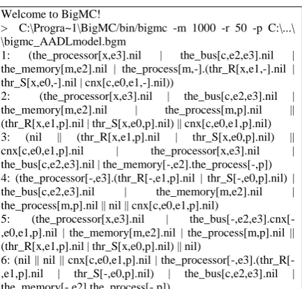
We choose to check the consistency and the correctness of the installation task. This must be verified by the satisfaction of all software-hardware components dependencies. In respect to our model, this may be ensured when bigraphs names disappear as x, m and c and software components are well deployed on hardware one. The property of consistency expressed in table 8 must be analyzed by the application of rules, expressed above in the same table. Table 9 shows the checking process steps. We can note that the successful state is achieved after 9 steps. This means that the consistency of installation task is valid.
Table 9. The checking results of the installation task.
Welcome to BigMC!
> C:\Progra~1\BigMC/bin/bigmc -m 1000 -r 50 -p C:\...\ \bigmc_AADLmodel.bgm
1: (the_processor[x,e3].nil | the_bus[c,e2,e3].nil | the_memory[m,e2].nil | the_process[m,-].(thr_R[x,e1,-].nil | thr_S[x,e0,-].nil | cnx[c,e0,e1,-].nil))
2: (the_processor[x,e3].nil | the_bus[c,e2,e3].nil | the_memory[m,e2].nil | the_process[m,p].nil || (thr_R[x,e1,p].nil | thr_S[x,e0,p].nil) || cnx[c,e0,e1,p].nil) 3: (nil || (thr_R[x,e1,p].nil | thr_S[x,e0,p].nil) || cnx[c,e0,e1,p].nil | the_processor[x,e3].nil | the_bus[c,e2,e3].nil | the_memory[-,e2].the_process[-,p]) 4: (the_processor[-,e3].(thr_R[-,e1,p].nil | thr_S[-,e0,p].nil) | the_bus[c,e2,e3].nil | the_memory[m,e2].nil | the_process[m,p].nil || nil || cnx[c,e0,e1,p].nil)
5: (the_processor[x,e3].nil | the_bus[-,e2,e3].cnx[-,e0,e1,p].nil | the_memory[m,e2].nil | the_process[m,p].nil || (thr_R[x,e1,p].nil | thr_S[x,e0,p].nil) || nil)
6: (nil || nil || cnx[c,e0,e1,p].nil | the_processor[-,e3].(thr_R[-,e1,p].nil | thr_S[-,e0,p].nil) | the_bus[c,e2,e3].nil | the_memory[-,e2].the_process[-,p])
7: (nil || (thr_R[x,e1,p].nil | thr_S[x,e0,p].nil) || nil | the_processor[x,e3].nil | the_bus[-,e2,e3].cnx[-,e0,e1,p].nil | the_memory[-,e2].the_process[-,p] )
8: (the_processor[-,e3].(thr_S[-,e0,p].nil | thr_R[-,e1,p].nil) | the_bus[-,e2,e3].cnx[-,e0,e1,p].nil | the_process[m,p].nil || nil || nil | the_memory[m,e2].nil)
9: (the_memory[-,e2].the_process[-,p].() | the_bus[-,e2,e3].cnx[-,e0,e1,p].nil | the_processor[-,e3].(thr_S[-,e0,p].nil | thr_R[-,e1,p].nil) | nil || nil || nil)
[mc::step] Complete!
[mc::report] [q: 0 / g: 9] @ 10
6.2.
Reconfiguration Checking
In the following table (Table 10), we present a bigraphical specification of the_process reconfiguration (having two threads thr_R1 and thr_R2). The rule expressed in the table 10, may permit to the_process component switching from thr_R1 to thr_R2. The purpose of the new added reaction rule (last one in table 10) is to allow the reconfiguration of the software component the_process as it is defined in AADL specification (table 6).
The BigMc tool tries to apply these reaction rules and reaches the state specified in the property clause. In our case, the reconfiguration property (reconf) is analyzed after 13 steps (see table 11).
Table 10. The BigMc reconfiguration property
#Nodes
%active the_processor : 2; %passive thr_S : 3; %passive thr_R1 : 3; %passive thr_R2 : 3; %...
#Links
%name x; %name m; %name p; %name c; %... #Sender/Receiver model
the_processor[x,e3] | the_bus[c,e2,e3] | the_memory[m,e2] | the_process[m,-].(thr_R1[x,e1,-] | thr_S[x,e0,-] | cnx[c,e0,e1,-];
#Reaction rules
the_process[m,-].(thr_R[x,e1,-] | thr_S[x,e0,-] | cnx[c,e0,e1,-]) -> the_process[m,p] || (thr_R[x,e1,p] | thr_S[x,e0,p]) || cnx[c,e0,e1,p;]
the_memory[m,e2].$0 || the_process[m,p] -> the_memory[-,e2].the_process[-,p].($1 | $2) || nil;
the_processor[x,e3].$2 || (thr_R[x,e1,p] | thr_S[x,e0,p]) ->
the_processor[-,e3].(thr_R[-,e1,p] | thr_S[-,e0,p]) || nil; the_bus[c,e2,e3].$1 || cnx[c,e0,e1,p] -> the_bus[-,e2,e3].cnx[-,e0,e1,p] || nil;
the_processor[-,e3].(thr_R[-,e1,p].nil | thr_S[-,e0,p].nil) -> the_processor[-,e3].(thr_R2[-,e1,p].nil | thr_S[-,e0,p].nil);
%property reconf (the_processor[-,e3].(thr_R2[-,e1,p].nil | thr_S[-,e0,p].nil) | the_bus[-,e2,e3].cnx[-,e0,e1,p].nil | the_memory[-,e2].the_process[-,p];
%check
specify and analyze deployment activities. Redundancies and inconsistencies caused by this diversity of formalisms may lead with difficulties in software application analysis and installation.
Table 11. The checking result of the reconfiguration task
Welcome to BigMC!
> C:\Progra~1 \bigmc_model.bgm
1: (the_processor[x,e3].nil | the_bus[c,e2,e3].nil |
the_memory[m,e2].nil | the_process[m,-].(thr_R1[x,e1,-].nil | thr_S[x,e0,-].nil | cnx[c,e0,e1,-].nil))
2: (the_processor[x,e3].nil | the_bus[c,e2,e3].nil |
the_memory[m,e2].nil | the_process[m,p].nil || (thr_R1[x,e1,p].nil | thr_S[x,e0,p].nil) || cnx[c,e0,e1,p].nil)
3: (nil || (thr_R1[x,e1,p].nil | thr_S[x,e0,p].nil) || cnx[c,e0,e1,p].nil | the_processor[x,e3].nil | the_bus[c,e2,e3].nil | the_memory[-,e2].the_process[-,p].())
4: (the_processor[x,e3].nil | the_bus[-,e2,e3].cnx[-,e0,e1,p].nil | the_memory[m,e2].nil | the_process[m,p].nil || (thr_R1[x,e1,p].nil | thr_S[x,e0,p].nil) || nil)
5: (the_processor[-,e3].(thr_R1[-,e1,p].nil | thr_S[-,e0,p].nil) | the_bus[c,e2,e3].nil | the_memory[m,e2].nil | the_process[m,p].nil || nil || cnx[c,e0,e1,p].nil)
6: (nil || (thr_R1[x,e1,p].nil | thr_S[x,e0,p].nil) || nil | the_processor[x,e3].nil | the_bus[-,e2,e3].cnx[-,e0,e1,p].nil | the_memory[-,e2].the_process[-,p].())
7: (nil || nil || cnx[c,e0,e1,p].nil | the_processor[-,e3].(thr_R1[-,e1,p].nil | thr_S[-,e0,p].nil) | the_bus[c,e2,e3].nil | the_memory[-,e2].the_process[-,p].())
8: (the_processor[-,e3].(thr_S[-,e0,p].nil | thr_R1[-,e1,p].nil) | the_process[m,p].nil || nil || nil | the_memory[m,e2].nil | the_bus[-,e2,e3].cnx[-,e0,e1,p].nil)
9: (the_bus[c,e2,e3].nil | the_processor[-,e3].(thr_S[-,e0,p].nil | thr_R2[-,e1,p].nil) | the_process[m,p].nil || nil || cnx[c,e0,e1,p].nil | the_memory[m,e2].nil)
10: (the_processor[-,e3].(thr_S[-,e0,p].nil | thr_R2[-,e1,p].nil) | the_memory[-,e2].the_process[-,p].() | the_bus[-,e2,e3].cnx[-,e0,e1,p].nil | nil || nil || nil)
11: (the_processor[-,e3].(thr_S[-,e0,p].nil | thr_R2[-,e1,p].nil) | nil || nil || cnx[c,e0,e1,p].nil | the_memory[-,e2].the_process[-,p].() | the_bus[c,e2,e3].nil)
12: (the_processor[-,e3].(thr_S[-,e0,p].nil | thr_R2[-,e1,p].nil) | the_process[m,p].nil || nil || nil | the_memory[m,e2].nil | the_bus[-,e2,e3].cnx[-,e0,e1,p].nil)
13: (the_memory[-,e2].the_process[-,p].() | the_bus[-,e2,e3].cnx[-,e0,e1,p].nil | the_processor[-,e3].(thr_S[-,e0,p].nil | thr_R2[-,e1,p].nil) | nil || nil || nil)
[mc::step] Complete!
[mc::report] [q: 0 / g: 13] @ 14
7.
CONCLUSION
The deployment of a software application on a specific execution environment is crucial and delicate stage that can guarantee its efficiency. In this paper, we proposed a mathematical model, based on BRS, allowing the modelling of the two deployment tasks, installation and reconfiguration of an AADL architectural application.
We have first defined a mapping between the architectural elements of AADL and those of bigraphs, offering generic transformation rules (meta-rules). Then, we have formalized the two AADL structures, application and runtime platform, contained in an AADL configuration declaration, by two distinct bigraphs GS and GH. These are composed to produce
a new bigraph showing the installation of the application on the runtime platform. AADL system reconfiguration was also formalized thanks to our BRS-based model, exploiting bigraphical reaction rules. Various and promising results were
obtained while validating our developed BRS-based model by the BigMc model checker.
In a subsequent work, we intend to automate the checking process of the installation and the reconfiguration of any AADL software application. We project also to enrich the properties set to check dynamically.
8. REFERENCES
[1] Medvidovic, N. and Taylor, R. N. 2000. A Classification and Comparison Framework for Software Architecture Description Languages. IEEE Tran. on Soft. Eng. 26(1):70-93.
[2] Zhang, P. Muccini, H. and Li, B. 2010. A classification and comparison of model checking software architecture techniques. Journal of Syst. Software. doi:10.1016/j.jss.
[3] Parrish, A. Dixon, B. and Cordes, D. 2001. A Conceptual Foundation for Component-Based Software Deployment. Journal of Systems and Software. 57(3): 193-200.
[4] SAE. International Avionics Systems Division (ASD). 2004. Avionics Architecture Description Language Standard. Available: http://www.sae.org.
[5] SEI. 2004. OSATE: An extensible Source AADL Tool Environment. SEI AADL Team technical Report.
[6] Lasnier, G. Zalila, B. Pautet, L. and Hugues, J. 2009. OCARINA: An Environment for AADL Models Analysis and Automatic Code Generation for High Integrity Applications. In Reliable Soft. Tech.’09 LNCS - Ada Europe, France. 237–250.
[7] Jensen, O.H. and Milner, R. 2004. Bigraphs and mobiles processes (revised). Technical Report 580, University of Cambridge, ISSN: 1476-2986.
[8] Chang, Z. X. M. and Qi, Z. 2007. An Approach based on Bigraphical Reactive Systems to Check Architectural Instance Conforming to its Style. First Joint IEEE/IFIP Symposium on Theoretical Aspects of Software Engineering (TASE'07). 57-66.
[9] Perrone, G. and Hildebrandt, T. 2012. A Model Checker for Bigraphs. In proceedings of the 27th ACM Sym. in Applied Computing ACM-SAC'12.
[10]Farail, P. Gaufillet, P. Canals, A. Camus, C. L. Sciamma, D. Michel, P. Crégut, X. and Pantel, M. 2006. TOPCASED: An Open Source Development Environment for Embedded Systems. MDD Concepts to Experiments and Illustrations, ISTE Editor.
[11]Milner, R. 2008. Bigraphs: a space for interaction. Available on web site: http://www.cl.cam.ac.uk.
[12]Conforti, G. Macedonio, D. and Sassone, V. 2005, BiLog: Spatial Logics for Bigraphs. In Proc. of the 32th ICALP’05, LNCS, Springer Verlag editor. 3580. 766-778.
[13]Bruni, R. Lafuente, A. L. Montanari,U. and Tuosto, E. 2007. Style-Based Architectural Reconfigurations. Bulletin of the European Association for Theoretical Computer Science, EATCS. 94:161-180.
[15]Allen, R. Douence R., and Garlan, D. 1998. Specifying and Analyzing Dynamic Software Architectures. In Proceedings of the 1998 Conf. on Fundamental Approaches to Soft. Eng. Lisbon, Portugal. 21-37. 11-79.
[16]Bures, T., Hnetynka, P. and Plasil, F. 2006. SOFA 2.0: Balancing Advanced Features in a Hierarchical Component Model. SERA, pp. 40-48.
[17]Belguidoum, M. and Dagnat, F. 2007. Dependency Management in Software Component Deployment. Electr. Notes Theor. Comput. Sci. (ENTCS) Vol. 182, pp.17-32.